Using the ccviR package • ccviR

Introduction

The ccviR package implements the NatureServe Climate Change Vulnerability Index (CCVI) in an R package and Shiny App. The package allows all of the geospatial aspects of calculating the CCVI to be done in R, removing the need for separate GIS calculations. It also enables easier sensitivity analysis of the Index.

The NatureServe CCVI is a trait based climate change vulnerability assessment framework. It includes three commonly used components of vulnerability: exposure, sensitivity and adaptive capacity. In addition, it optionally incorporates the results of documented or modeled responses to climate change.

Exposure is assessed by determining the proportion of the species range that falls into 6 classes of temperature and moisture change which is used to assign an exposure multiplier. Sensitivity and adaptive capacity are assessed by scoring 23 vulnerability factors, on a scale from 0 (‘neutral’) to 3 (‘greatly increases vulnerability’). These scores are then multiplied by the exposure multiplier and are summed to give a total score for this section. Factors that cannot be answered can be left blank and contribute 0 to the total score. If fewer than 13 factors are scored the index value cannot be calculated.

In addition, there are 4 vulnerability factors for documented or modeled responses to climate change that can optionally be scored on a similar scale. These scores are simply summed to get the total score for this section. An index value is then determined for the two sections (exposure x sensitivity and adaptive capacity, and documented or modeled responses) by applying a set of thresholds to the scores. The two index values are then combined using a table that gives more weight to the sensitivity and adaptive capacity section. The possible index values are Less Vulnerable, Moderately Vulnerable, Highly Vulnerable, Extremely Vulnerable or Insufficient Evidence (if not enough factors of the CCVI are scored). For more detailed information on how the index works and how each factor is scored see the NatureServe CCVI Guidelines and the references below.

Getting started

To begin using the ccviR package within R, you will need to load the required packages. An example data set has been provided within the package that we will use in the examples below. The prepared data will be saved in the output folder and can be used whenever the index is being calculated, so this step only needs to be completed once. The following code block loads the required packages and the example data set:

#load packages
library(ccviR)
library(sf)
#> Linking to GEOS 3.10.2, GDAL 3.4.1, PROJ 8.2.1; sf_use_s2() is TRUE
library(dplyr)
#> 
#> Attaching package: 'dplyr'
#> The following objects are masked from 'package:stats':
#> 
#>     filter, lag
#> The following objects are masked from 'package:base':
#> 
#>     intersect, setdiff, setequal, union

#load example data set
data_pth <- system.file("extdata", package = "ccviR")

Preparing the climate data

This step is only necessary if you want to use custom climate data. You can skip this section if you are using pre-prepared climate data which is available for download here.

Step 1: Acquire climate data. We recommend the climate data for North America from AdaptWest but any data set that includes at least the mean annual temperature and climate moisture deficit (or a similar moisture metric) can be used. For AdaptWest select the bioclimatic variables for the normal period and the desired future climate scenario. We recommend using the 1961-1990 normal period and the ensemble data for SSP2-4.5 and SSP5-8.5 for the 2050s for the future. Accepted raster file types are “.asc”, “.tif”, “.nc”, “.grd” and “.img”. Save the downloaded data in a folder you can easily find.

Step 2: Prepare the climate data for use in ccviR. Climate data can be processed by providing file paths for each file or for a folder that contains all the files with standard names. For the output folder, make sure to choose a location that is easy to find again because you will use the prepared climate data to calculate the index. When preparing data for multiple scenarios, you will need to process each scenario separately but save the thresholds used to classify the first scenario and supply them when processing subsequent scenarios (this is demonstrated in the example below).

Standard names for input folder:

MAT: mean annual temperature for the historical normal period (required)
MAT_2050: mean annual temperature for the future under climate change. It can be any number eg 2050, 2100 (required)
CMD: climate moisture deficit for the historical normal period (required)
CMD_2050: climate moisture deficit for the future under climate change it can be any number eg 2050, 2100 (required)
CCEI: Climate Change Exposure Index from NatureServe website
MAP: mean annual precipitation for the historical normal period
MWMT: mean warmest month temperature for the historical normal period
MCMT: mean coldest month temperature for the historical normal period
clim_poly: An optional shapefile with a polygon of the extent of the climate data. It will be created from the climate data if it is missing but it is faster to provide it.

The thresholds for classifying data are based on those provided in the NatureServe Guidelines except for the thresholds used for the exposure data. Since we are using different climate data the thresholds for the classes need to be calculated. We use the the median and 1/2 the interquartile range since it is more appropriate for skewed data than the mean and standard deviation which are used by NatureServe for the continental US.

The following code prepares the climate data from the example data set using prep_clim_data:

# climate data file names
list.files(file.path(data_pth, "clim_files/raw"))
#> [1] "NB_norm_CMD.tif"    "NB_norm_MAP.tif"    "NB_norm_MAT.tif"   
#> [4] "NB_norm_MCMT.tif"   "NB_norm_MWMT.tif"   "NB_RCP.4.5_CMD.tif"
#> [7] "NB_RCP.4.5_MAT.tif" "NB_RCP.8.5_CMD.tif" "NB_RCP.8.5_MAT.tif"

# prepare the data and save it in out_folder
# RCP4.5 prep - saves breaks as brks for use in 8.5 prep
brks <- prep_clim_data(
  mat_norm = file.path(data_pth, "clim_files/raw", "NB_norm_MAT.tif"),
  mat_fut = file.path(data_pth, "clim_files/raw", "NB_RCP.4.5_MAT.tif"),
  cmd_norm = file.path(data_pth, "clim_files/raw", "NB_norm_CMD.tif"),
  cmd_fut = file.path(data_pth, "clim_files/raw", "NB_RCP.4.5_CMD.tif"),
  map = file.path(data_pth, "clim_files/raw", "NB_norm_MAP.tif"),
  mwmt = file.path(data_pth, "clim_files/raw", "NB_norm_MWMT.tif"),
  mcmt = file.path(data_pth, "clim_files/raw", "NB_norm_MCMT.tif"),
  clim_poly = file.path(data_pth, "clim_files/processed", "clim_poly.shp"),
  out_folder = file.path(data_pth, "clim_files/processed"),
  overwrite = TRUE,
  scenario_name = "RCP 4.5",
)
#> processing MAT
#> processing CMD
#> processing MAP
#> processing MWMT and MCMT
#> finished processing

# RCP8.5 - using breaks from 4.5
# map, mwmt and mcmt only need to be processed once
prep_clim_data(
  mat_norm = file.path(data_pth, "clim_files/raw", "NB_norm_MAT.tif"),
  mat_fut = file.path(data_pth, "clim_files/raw", "NB_RCP.8.5_MAT.tif"),
  cmd_norm = file.path(data_pth, "clim_files/raw", "NB_norm_CMD.tif"),
  cmd_fut = file.path(data_pth, "clim_files/raw", "NB_RCP.8.5_CMD.tif"),
  out_folder = file.path(data_pth, "clim_files/processed"),
  clim_poly = file.path(system.file("extdata", package = "ccviR"),
                        "assess_poly.shp"),
  overwrite = TRUE,
  scenario_name = "RCP 8.5",
  brks_mat = brks$brks_mat, 
  brks_cmd = brks$brks_cmd,
  brks_ccei = brks$brks_ccei
)
#> processing MAT
#> processing CMD
#> finished processing

Using the mean annual temperature (MAT) as an example, we will explore how the data is prepared. prep_clim_data determines the change in MAT and classifies it into six classes (1-6) where 6 has the largest increase in temperature. The thresholds, or breaks, for classifying data are based on those provided in the NatureServe Guidelines (except for the thresholds used for the exposure data). Since custom climate data is being used, the thresholds for the classes need to be calculated. To calculate the thresholds we use the the median and 1/2 the interquartile range. These values are more appropriate for skewed data than the mean and standard deviation which are used by NatureServe for the continental US.

The change in MAT and the classified MAT (output from prep_clim_data) can be plotted to demonstrate the classification of the change in MAT.

# select color ramp for plots
pal = c("#FFF9CA", "#FEE697", "#FEC24D", "#F88B22", "#D85A09", "#A33803")

# create rasters for the historical normal MAT and the future MAT
mat_norm <- terra::rast(file.path(data_pth, "clim_files/raw/NB_norm_MAT.tif"))
mat_fut <- terra::rast(file.path(data_pth, "clim_files/raw/NB_RCP.4.5_MAT.tif"))

# plot the change in MAT
terra::plot(mat_norm - mat_fut, 
     col = colorRampPalette(rev(pal))(50))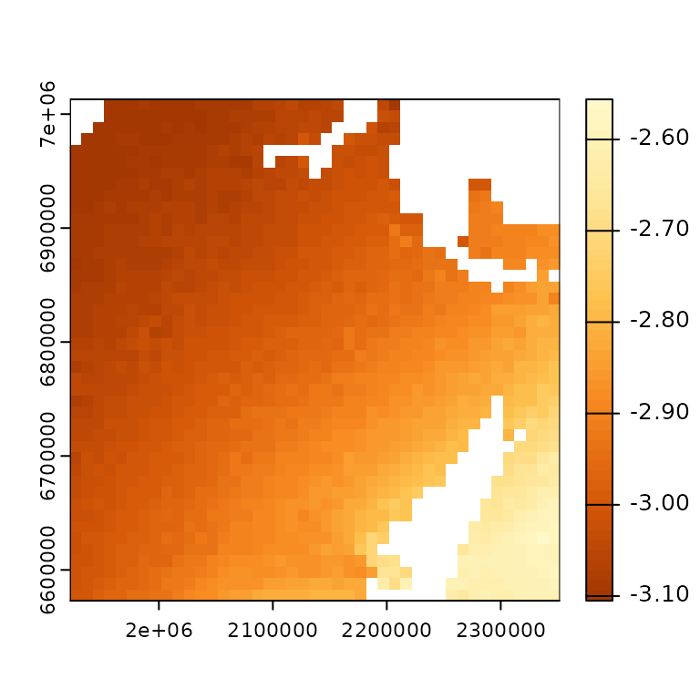

# breaks used to classify data (determined when preparing RCP4.5 data above)
brks$brks_mat
#>        [,1]   [,2] [,3]
#> [1,] -4.105 -3.130    6
#> [2,] -3.130 -3.050    5
#> [3,] -3.050 -2.970    4
#> [4,] -2.970 -2.890    3
#> [5,] -2.890 -2.810    2
#> [6,] -2.810 -1.556    1

# create raster for the classified MAT
mat_classified <- terra::rast(file.path(data_pth, "clim_files/processed/MAT_reclassRCP_4.5.tif"))

# plot the classified MAT
terra::plot(mat_classified, col = pal)

Note that the plot only shows five classes as none of the data falls within the sixth class.

When preparing custom climate data, it is recommended that a csv readme file is created and stored to record where the data came from and any relevant metadata. This file is required if the data is used with the ccviR Shiny app.

# make readme csv
write.csv(
  data.frame(Scenario_Name = c("RCP 4.5", "RCP 8.5"),
             GCM_or_Ensemble_name = "AdaptWest 15 CMIP5 AOGCM Ensemble",
             Historical_normal_period = "1961-1990",
             Future_period = "2050s",
             Emissions_scenario = c("RCP 4.5", "RCP8.5"),
             Link_to_source = "https://adaptwest.databasin.org/pages/adaptwest-climatena-cmip5/",
             brks_mat = brks$brks_mat %>% brks_to_txt(),
             brks_cmd = brks$brks_cmd %>% brks_to_txt(),
             brks_ccei = brks$brks_ccei %>% brks_to_txt()),
  file.path(data_pth, "clim_files/processed/", "climate_data_readme.csv"),
  row.names = FALSE
)

Load species specific spatial data

The following spatial data sets can be input for each species:

Species North American or global range polygon (required)
Assessment area polygon (required)
Non-breeding range polygon
Projected range change raster and a matrix to reclassify it as 0 = unsuitable, 1 = lost, 2 = maintained and 3 = gained
Physiological thermal niche (PTN) polygon. PTN polygon should include cool or cold environments that the species occupies that may be lost or reduced in the assessment area as a result of climate change.

See here for more details on these spatial inputs. For this example all of the data is provided with the package.

rng_poly <- read_sf(file.path(data_pth, "rng_poly.shp"), agr = "constant")
assess_poly <- read_sf(file.path(data_pth, "assess_poly.shp"), agr = "constant")
rng_chg <- terra::rast(c(file.path(data_pth, "rng_chg_45.tif"), 
                 file.path(data_pth, "rng_chg_85.tif")))
PTN_poly <- read_sf(file.path(data_pth, "PTN_poly.shp"), agr = "constant")

# the range change raster has values from -1, 0 and 1, this matrix is used to
# convert them to the 4 classes described above.
hs_rcl_mat <- matrix(c(-1:1, c(1, 2, 3)), ncol = 2)

Load climate data

Next we will load in the climate data that we prepared in the first step using the get_clim_vars() function which loads the data and stores it in a list with the required names. The scenario names must match the suffix on the file name which is done automatically by prep_clim_data. The result is a list where each element is a single layer SpatRaster for static variables and a multi-layer SpatRaster for variables that change, with one layer per scenario. The clim_poly is also included as an sf object.

clim_dat <- get_clim_vars(file.path(data_pth, "clim_files/processed"), 
                          scenario_names = c("RCP 4.5", "RCP 8.5"))

str(clim_dat, max.level = 1)
#> List of 6
#>  $ mat      :S4 class 'SpatRaster' [package "terra"]
#>  $ cmd      :S4 class 'SpatRaster' [package "terra"]
#>  $ map      :S4 class 'SpatRaster' [package "terra"]
#>  $ ccei     : NULL
#>  $ htn      :S4 class 'SpatRaster' [package "terra"]
#>  $ clim_poly:Classes 'sf' and 'data.frame':  1 obs. of  11 variables:
#>   ..- attr(*, "sf_column")= chr "geometry"
#>   ..- attr(*, "agr")= Factor w/ 3 levels "constant","aggregate",..: 1 1 1 1 1 1 1 1 1 1
#>   .. ..- attr(*, "names")= chr [1:10] "GID_0" "NAME_0" "GID_1" "NAME_1" ...

Run spatial data analysis

Once the species specific and climate data is loaded, we can run the spatial data analysis:

spat_res <- analyze_spatial(range_poly = rng_poly, scale_poly = assess_poly,
                            clim_vars_lst = clim_dat, ptn_poly = PTN_poly,
                            hs_rast = rng_chg, hs_rcl = hs_rcl_mat, 
                            scenario_names = c("RCP 4.5", "RCP 8.5"))
#> performing spatial analysis
#> Warning: More than 10% of the range change raster does not match the expected values.
#> Is the classification table correct?

The resulting object is a list containing a table with the results of the spatial analysis (spat_res$spat_table) and two range polygons which are provided for mapping (spat_res$range_poly_assess and spat_res$range_poly_clim). In this case, spat_res$spat_table shows that the range is spread over the 2nd, 3rd and 4th highest exposure classes for change in MAT:

spat_res$spat_table[, 1:7]
#>   scenario_name MAT_1 MAT_2 MAT_3  MAT_4 MAT_5 MAT_6
#> 1       RCP 4.5     0     0 8.067 64.113 27.82     0
#> 2       RCP 8.5     0     0 0.000  0.000  0.00   100

spat_res$range_poly_assess is the range polygon clipped to the assessment area while spat_res$range_poly_clim is the range polygon clipped to the extent of the climate data. spat_res$range_poly_assess is used for all factors except the historical thermal and hydrological niche which use spat_res$range_poly_clim. This is because the historical thermal and hydrological niche are used as proxies for the range of temperature and moisture conditions that the species can tolerate and, therefore, should reflect as much of the range as possible. If the range polygon provided is completely within the assessment area then spat_res$range_poly_assess will be the same as the provided range polygon.

We can create a map to visualize the exposure to changes in MAT for the RCP 4.5 scenario by overlaying the range clipped to the assessment area on top of the change in MAT raster:

terra::plot(clim_dat$mat$RCP_4.5, col = pal)

plot(st_geometry(spat_res$range_poly_assess), add = TRUE)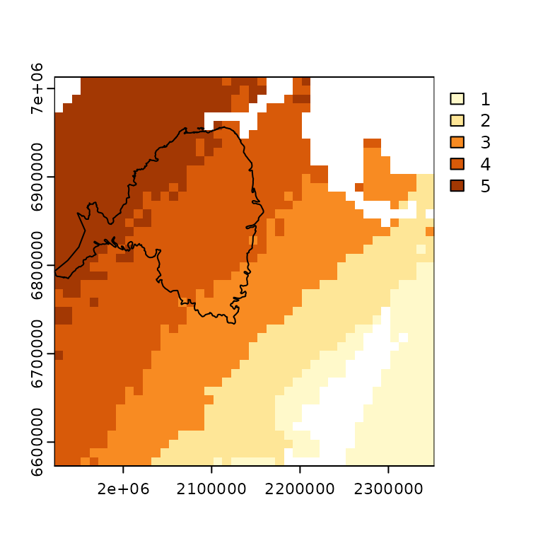

Answer the vulnerability questions

make_vuln_df() creates a blank table that can be filled in with scores for each vulnerability factor used to calculate the index. The vulnerability factors and how to score them is explained in the NatureServe CCVI Guidelines. The table includes an abbreviated version of the question ($Question), the maximum value for each factor ($Max_Value), and whether the factor is calculated by the spatial data analysis ($is_spatial). When the factor is calculated by the spatial analysis, indicated by $is_spatial != NA, it should be scored as -1 so as not to override the results of the spatial analysis.

# create a blank vulnerability question table
vuln <- make_vuln_df("sp_name")

$Value1 should be filled with the number corresponding to the following impacts on vulnerability -1: Unknown, 0: Neutral, 1: Somewhat Increase, 2: Increase, 3: Greatly Increase. Note that the maximum Value1 value depends on the question, it can be 2 or 3 (reflected by $Max_Value). If you wish to input two or more answers to reflect uncertainty you do so by filling in $Value2, $Value3, and/or $Value4. The table can be filled out interactively, using code (recommended for reproduceability), or by saving the table as a csv, editing it, and loading it back into R. These three options are outlined in the codeblocks below:

Interactive editing:

# you can interactively edit the table
vuln <- edit(vuln)

Editing using code:

# or use code (recommended for reproducibility)
vuln$Value1[3:19] <- c(0, 0, 1, 0, -1, -1, -1, -1, 0, 0, 1, 0, 0, 1, 0, 0, 0)
vuln$Value1[26:29] <- c(0, -1, -1, 0)

# include a second value to reflect uncertainty and trigger a monte carlo to
# determine confidence
vuln$Value2[3:5] <- c(2, 0, 0)

Editing using a csv:

# save the table as a csv 
write.csv(vuln, "path/to/write", row.names = FALSE)

# edit the csv and save it 
# load it back in to R
vuln <- read.csv("path/to/write", stringsAsFactors = FALSE)

Calculate the index

Finally, use the results of the spatial analysis and the answers to the vulnerability questions to calculate the index. For this example the number of rounds in the Monte Carlo has been reduced but it should generally be kept to the default (n_rnds = 1000).

index_res <- calc_vulnerability(spat_res$spat_table, vuln, tax_grp = "Bird",
                                n_rnds = 20)
#> calculating vulnerability index RCP 4.5
#> performing monte carlo
#> finished vulnerability
#> calculating vulnerability index RCP 8.5
#> performing monte carlo
#> finished vulnerability

The result is a dataframe with 12 columns (see ?calc_vulnerability for an explanation of all of them). $index gives the index where EV: Extremely Vulnerable, HV: Highly Vulnerable, MV: Moderately Vulnerable, LV: Less Vulnerable, and IE: Insufficient Evidence. Below we see that our example species is Highly Vulnerable to climate change:

glimpse(index_res)
#> Rows: 2
#> Columns: 12
#> $ scenario_name <chr> "RCP 4.5", "RCP 8.5"
#> $ index         <chr> "HV", "EV"
#> $ conf_index    <chr> "Low", "Very High"
#> $ mc_results    <list> [<tbl_df[20 x 5]>], [<tbl_df[20 x 5]>]
#> $ mig_exp       <chr> "N/A", "N/A"
#> $ d_score       <dbl> 4, 4
#> $ b_c_score     <dbl> 9.45, 12.05
#> $ vuln_df       <list> [<tbl_df[29 x 12]>], [<tbl_df[29 x 12]>]
#> $ n_b_factors   <int> 4, 4
#> $ n_c_factors   <int> 11, 11
#> $ n_d_factors   <int> 4, 4
#> $ slr_vuln      <lgl> FALSE, FALSE

index_res$index
#> [1] "HV" "EV"

We can investigate how the index value was reached using the results of calc_vulnerability and two graphs included in the package.

The first graph is plot_score_index(). It shows how the index values (that are calculated separately for the modeled response to climate change and sensitivity and adaptive capacity modified by exposure sections) are combined into the overall index value. It also shows where the thresholds are for converting the numerical scores from each factor into the categorical index value. In this example, we can see that the index value is driven primarily by the sensitivity section since the score in that section would have produced an index value of Extremely Vulnerable if the D score were higher or not included (-1 in the graph).

# set theme
my_theme <- ggplot2::theme_classic() +
  ggplot2::theme(text = ggplot2::element_text(size = 12),
                 strip.background = ggplot2::element_blank())

ggplot2::theme_set(my_theme)

plot_score_index(index_res)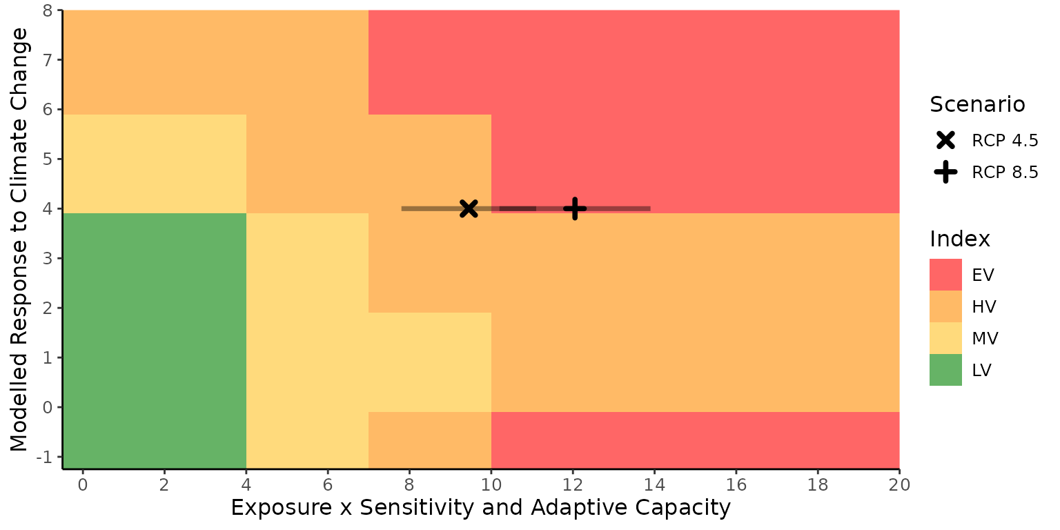

The second graph is produced by plot_q_score(). It is a plotly graph of the scores for each factor. The bars show the total score for the factor. The popup shows the name of the question and the exposure multiplier that was used to modify the score for the vulnerability factor.

q_score <- bind_rows(index_res$vuln_df %>% `names<-`(index_res$scenario_name), 
            .id = "scenario_name") %>%
  plot_q_score()

q_score

Since the output of the analysis is a data frame it can be saved and used to compare the results for multiple species or to test the sensitivity of the index to different inputs.