Plot bivariate exposure map

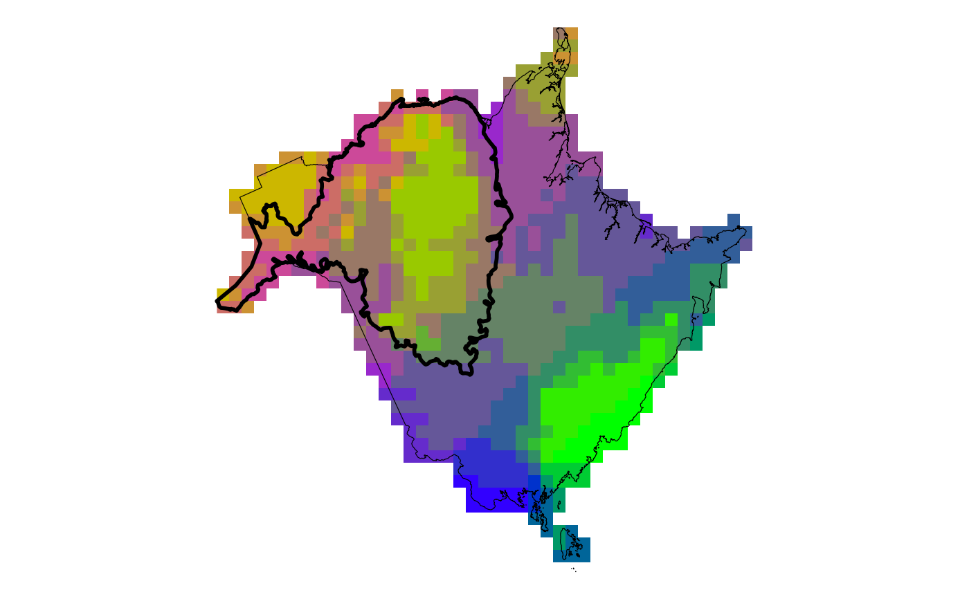
Create a map of exposure to climate change based on both change in temperature and change in climate moisture deficit.

Usage

plot_bivar_exp(
  mat,
  cmd,
  scale_poly,
  rng_poly = NULL,
  leg_rel_size = 2.5,
  palette = c(bottomleft = "green", bottomright = "blue", upperleft = "orange",
    upperright = "magenta")
)

Arguments

mat

RasterLayer of classified mean annual temperature exposure.

cmd

RasterLayer of classified climate moisture deficit exposure.

scale_poly

sf polygon of the assessment area.

rng_poly

sf polygon of the species range. Optional.

leg_rel_size

numeric, shrinkage of the legend size relative to the plot. Default is 2.5 larger numbers will make the legend smaller

palette

named vector of colours in each corner of the bivariate scale. Required names are bottomleft, bottomright, upperleft, and upperright.

Value

a list containing 2 ggplot objects "plot" containing the exposure map and "legend" containing the legend

Examples

# load the demo data
file_dir <- system.file("extdata", package = "ccviR")

# scenario names
scn_nms <- c("RCP 4.5", "RCP 8.5")

clim_vars <- get_clim_vars(file.path(file_dir, "clim_files/processed"),
                           scn_nms)

mat <- clim_vars$mat$RCP_4.5
cmd <- clim_vars$cmd$RCP_4.5

assess <- sf::st_read(file.path(file_dir, "assess_poly.shp"), agr = "constant",
                  quiet = TRUE)
rng <- sf::st_read(file.path(file_dir, "rng_poly.shp"), agr = "constant",
               quiet = TRUE)

plot_bivar_exp(mat, cmd, assess, rng)
#> Preparing polygon 'assessment area polygon'
#> Preparing polygon 'assessment area polygon'
#> $plot

#> 
#> $legend

#>