Caribou Demographic Rates and Trajectories

1 Demographic rates and trajectories from the national model

1.1 Overview

Here we describe a demographic model with density dependence and interannual variability following Johnson et al. (2020) with modifications noted in Hughes et al. (2025) and Dyson et al. (2026). Demographic rates vary with disturbance as estimated by Johnson et al. (2020). A detailed description of the model is provided in (Hughes et al. 2025, sec. 2.4).

getNationalCoefficients() selects the regression coefficient values and standard errors for the desired model version (see popGrowthTableJohnsonECCC for options) and then samples coefficients from these Gaussian distributions for each replicate population.

Next estimateNationalRates() is used to apply the sampled coefficients to the disturbance covariates to calculate expected recruitment and survival according to the beta regression models estimated by Johnson et al. (2020). Each population is optionally assigned to quantiles of the Beta error distributions for survival and recruitment. Using quantiles means that the population will stay in these quantiles as disturbance changes over time, so there is persistent variation in recruitment and survival among example populations.

Finally, we can use the estimated demographic rates to project population dynamics using a simple model with two age classes. Interannual variation in survival and recruitment is modelled using truncated Beta distributions.

library(bboutools)
library(caribouMetrics)
# use local version on local and installed on GH
if (requireNamespace("devtools", quietly = TRUE)) devtools::load_all()
library(dplyr)
library(ggplot2)
library(tidyr)
library(patchwork)

theme_set(theme_bw())
pthBase <- system.file("extdata", package = "caribouMetrics")

figWidth <- 8; figHeight <- 10

1.2 Demographic outcomes in a simple case no variation in disturbance over time or among populations

A simple case for demographic projection is multiple stochastic projections from a single landscape that does not change over time. First we define a disturbance scenario with 40% anthropogenic disturbance and 2% fire disturbance. If we had spatial data for the disturbance in our area of interest we could use disturbanceMetrics() to directly calculate the disturbance. See Disturbance Metrics vignette for an example.

disturbance <- data.frame(Anthro = 40, Fire_excl_anthro = 2)

We begin by sampling coefficients for 500 replicate populations using default Johnson et al. (2020) models “M1” and “M4”. The returned object is a list containing the coefficients and standard errors from the national model as well as the sampled coefficients and the quantiles that they have been assigned to.

popGrowthPars <- getNationalCoefficients(500)

head(popGrowthPars$coefSamples_Survival$coefSamples)
#>       Intercept        Anthro Precision
#> [1,] -0.1530718 -0.0008907556  60.65168
#> [2,] -0.1399809 -0.0007155384  61.65165
#> [3,] -0.1612743 -0.0007628660  68.57570
#> [4,] -0.1420441 -0.0007747503  52.81483
#> [5,] -0.1370847 -0.0009535161  52.68192
#> [6,] -0.1329182 -0.0008050787  60.32032
head(popGrowthPars$coefSamples_Survival$coefValues)
#>    Intercept Anthro Precision
#>        <num>  <num>     <num>
#> 1:    -0.142 -8e-04  63.43724
head(popGrowthPars$coefSamples_Survival$coefStdErrs)
#>      Intercept      Anthro Precision
#>          <num>       <num>     <num>
#> 1: 0.007908163 0.000127551  8.272731
head(popGrowthPars$coefSamples_Survival$quantiles)
#> [1] 0.25345691 0.02880762 0.89123246 0.36007014 0.55806613 0.19063126

Next we calculate sample demographic rates given sampled model coefficients and disturbance metrics for our example landscape, setting returnSample = TRUE so that the results returned contain a row for each sample in each scenario. We set the initial population size for each sample population to 100, and project population dynamics for 20 years using the caribouPopGrowth function with default parameter values. Anthropogenic disturbance is high on this example landscape, so the projected population growth rate for most sample populations is below 1, but there is variability in the model so few sample populations persist (Figure 1.1). If no initial population size is provided, the projections do not include population size, and realized population growth rate includes interannual variation but not density dependence or demographic stochasticity (Figure 1.2).

rateSamples <- estimateNationalRates(
  covTable = disturbance,
  popGrowthPars = popGrowthPars,
  ignorePrecision = FALSE,
  returnSample = TRUE,
  useQuantiles = FALSE)     
rateSamples$N0 <- 100
demography <- cbind(rateSamples,
                    caribouPopGrowth(N = rateSamples$N0,
                                     numSteps = 20,
                                     R_bar = rateSamples$R_bar,
                                     S_bar = rateSamples$S_bar))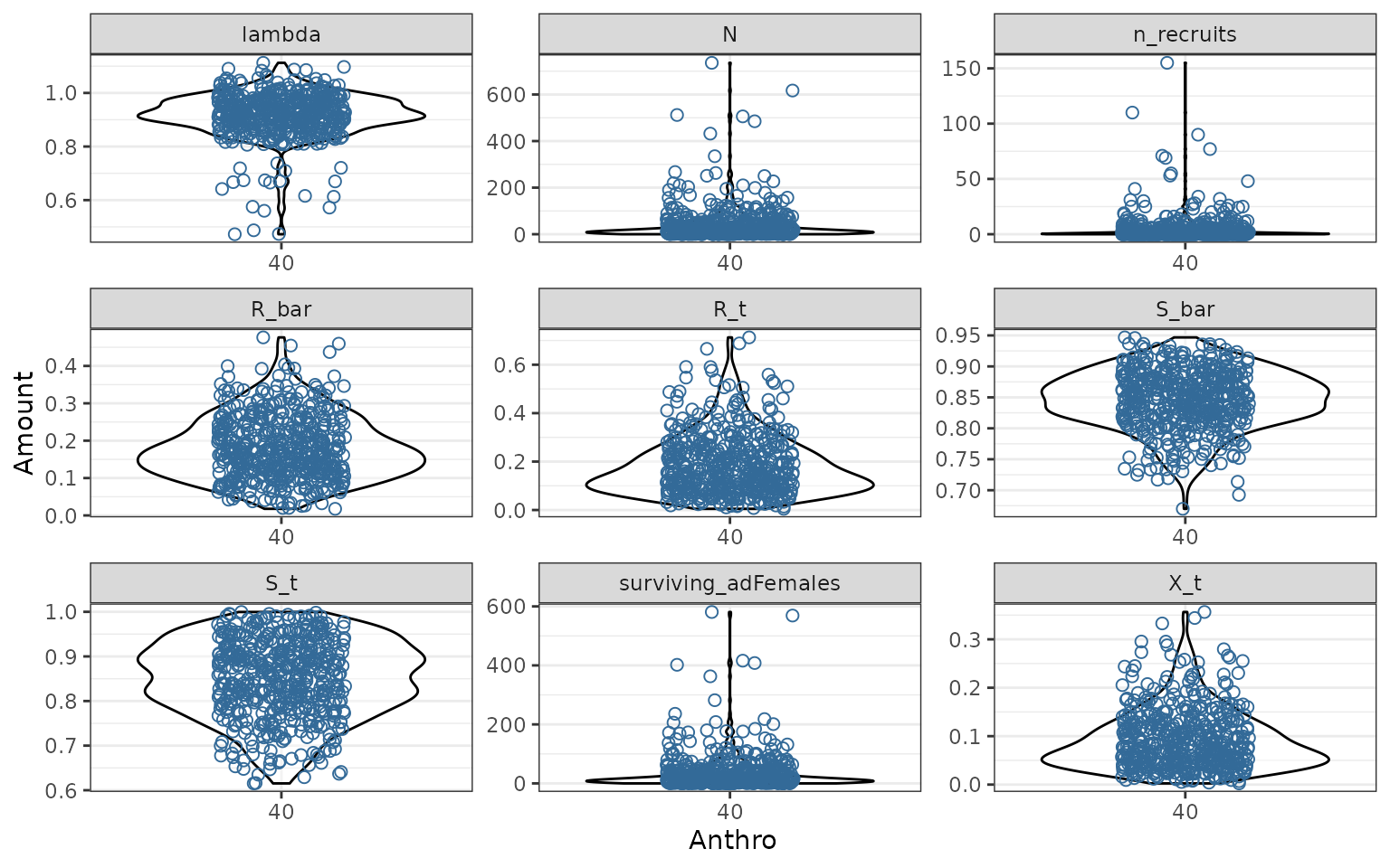

Figure 1.1: Variation in demographic rates and outcomes among 500 sample populations after a 20 year projection. Anthropogenic disturbance is 40%, fire disturbance is 2%. ‘lambda’ is realized population growth rate in the final year, and ‘lambdaE’ is expected population growth rate without interannual variation, density dependence or demographic stochasticity. ‘N’ is the number of adult females, which includes new recruits ‘n_recruits’ and survivors ‘surviving_adFemales’ from the previous year. ‘R_bar/S_bar’ are the expected recruitment (calf:cow ratio) and survival rates, ‘R_t/S_t’ are the recruitment and survival rates in the final year, which are more variable because they include interannual variation. ‘X_t’ is the recruitment rate adjusted for sex ratio and (optionally) composition survey bias - see Hughes et al. (2025) for details.

rateSamples$N0 <- NA
demography <- cbind(rateSamples,
                    caribouPopGrowth(N = rateSamples$N0,
                                     numSteps = 20,
                                     R_bar = rateSamples$R_bar,
                                     S_bar = rateSamples$S_bar))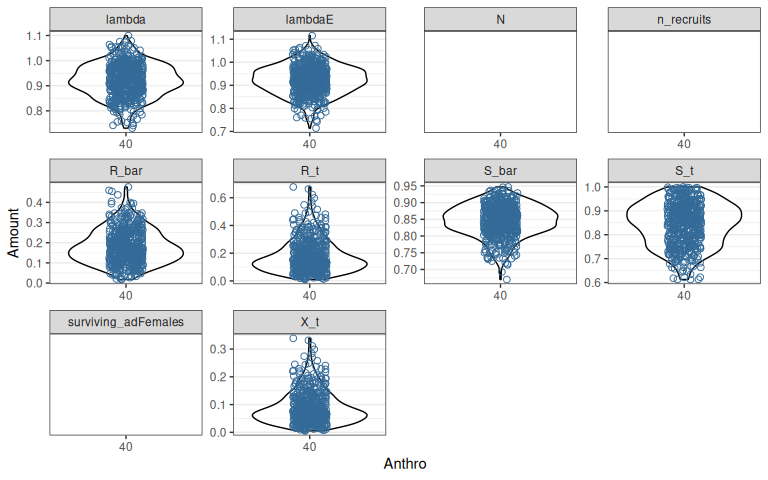

Figure 1.2: Variation in demographic rates and outcomes among 500 sample populations after a 20 year projection with no initial population size. See Figure 1.1 for other details.

1.3 Expected recruitment and survival: effects of disturbance and variation among populations

We can project demographic rates over a range of landscape conditions to recreate figures 3 and 5 from Johnson et al. (2020) and see the effects of changing disturbance on expected recruitment and survival. First we create a table of disturbance scenarios across a range of different levels of fire and anthropogenic disturbance.

covTableSim <- expand.grid(Anthro = seq(0, 90, by = 2), 
                           Fire_excl_anthro = seq(0, 70, by = 10)) 
covTableSim$Total_dist = covTableSim$Anthro + covTableSim$Fire_excl_anthro

We again sample coefficients from default models M1 and M4. The sample of 500 is used to calculate averages, while the sample of 35 is used to show variability among populations.

# set seed so vignette looks the same each time
set.seed(34533)

popGrowthPars <- getNationalCoefficients(
  500,
  modelVersion = "Johnson",
  survivalModelNumber = "M1",
  recruitmentModelNumber = "M4",
  populationGrowthTable = popGrowthTableJohnsonECCC
)

popGrowthParsSmall <- getNationalCoefficients(
  35,
  modelVersion = "Johnson",
  survivalModelNumber = "M1",
  recruitmentModelNumber = "M4",
  populationGrowthTable = popGrowthTableJohnsonECCC
)

Next we calculate expected survival and recruitment rates given sampled model coefficients. For the smaller sample we set returnSample = TRUE so that the results returned contain a row for each sample in each scenario. Setting useQuantiles = TRUE assigns each sample population to a quantile of the regression model error distributions for survival and recruitment, allowing variation among populations to persist as disturbance changes. For the larger sample we set returnSample = FALSE to get summaries of mean and variation across the samples.

Johnson et al’s (2020) Beta regression models estimate uncertainty about intercept and slope coefficients, and a precision parameter that describes variation among observations (Ferrari and Cribari-Neto 2004). To show the importance of considering both these sources of variation we compare results with ignorePrecision = TRUE and ignorePrecision = FALSE. If the goal is to estimate and visualize nationally applicable demographic-disturbance relationships then the precision parameter may not be of interest (Figure 1.3). If we are interested in the distribution of variation across the country it is essential to include both uncertainty about the regression coefficients and additional variation summarized by the precision parameter of the Beta regression model (Figure 1.4).

rateSamples <- estimateNationalRates(
  covTable = covTableSim,
  popGrowthPars = popGrowthParsSmall,
  ignorePrecision = FALSE,
  returnSample = TRUE,
  useQuantiles = TRUE
)

rateSummaries <- estimateNationalRates(
  covTable = covTableSim,
  popGrowthPars = popGrowthPars,
  ignorePrecision = FALSE,
  returnSample = FALSE,
  useQuantiles = FALSE
)

rateSummariesIgnorePrecision <- estimateNationalRates(
  covTable = covTableSim,
  popGrowthPars = popGrowthPars,
  ignorePrecision = TRUE,
  returnSample = FALSE,
  useQuantiles = FALSE
)

Figure 1.3: Variation in expected survival and recruitment with disturbance. Bands (2.5% and 97.5% quantiles of 500 samples) show variation due to uncertainty about intercept and slope coefficients in Johnson et al’s (2020) Beta regression models.

Figure 1.4: Variation in expected survival and recruitment with disturbance. Bands (2.5% and 97.5% quantiles of 500 samples) include both uncertainty about the regression coefficients and additional variation summarized by the precision parameter of Johnson et al’s (2020) Beta regression models. Faint coloured lines show example trajectories of expected demographic rates in sample populations, assuming each sample population is randomly distributed among quantiles of the beta distribution, and each population remains in the same quantile of the Beta distribution as disturbance changes.

1.4 Projection of population growth over time on a changing landscape: workflow details

In this example, we project 35 sample populations for 50 years on a landscape where the anthropogenic disturbance footprint is increasing by 5% per decade (Figure 1.5). Note the form of the growth model (density dependence, interannual variation, demographic stochasticity etc) can be changed by setting caribouPopGrowth() function parameters.

numTimesteps <- 50
stepLength <- 1
N0 <- 100
AnthroChange <- 5/10 #For illustration assume 5% increase in anthropogenic disturbance footprint each decade

# at each time,  sample demographic rates and project, save results
pars <- data.frame(N0 = N0)
for (t in 1:numTimesteps) {
  covariates <- disturbance
  covariates$Anthro <- covariates$Anthro + AnthroChange * (t - 1)

  rateSamples <- estimateNationalRates(
    covTable = covariates,
    popGrowthPars = popGrowthParsSmall,
    ignorePrecision = FALSE,
    returnSample = TRUE,
    useQuantiles = TRUE
  )
  if (hasName(pars,"N")) {
    pars <- subset(pars, select = c(replicate, N))
    names(pars)[names(pars) == "N"] <- "N0"
  }
  pars <- merge(pars, rateSamples)
  pars <- cbind(pars, 
                caribouPopGrowth(pars$N0,
                                 R_bar = pars$R_bar, S_bar = pars$S_bar,
                                 numSteps = stepLength))

  # add results to output set
  fds <- subset(pars, select = c(replicate, Anthro, N, S_bar,S_t, R_bar,R_t,lambdaE,lambda))
  fds$replicate <- as.numeric(gsub("V", "", fds$replicate))
  fds <- pivot_longer(fds, !replicate, names_to = "MetricTypeID", values_to = "Amount")
  fds$Timestep <- t * stepLength
  if (t == 1) {
    popMetrics <- fds
  } else {
    popMetrics <- rbind(popMetrics, fds)
  }
}

popMetrics$MetricTypeID <- as.character(popMetrics$MetricTypeID)
popMetrics$Replicate <- paste0("x", popMetrics$replicate)
# popMetrics <- subset(popMetrics, !MetricTypeID == "N")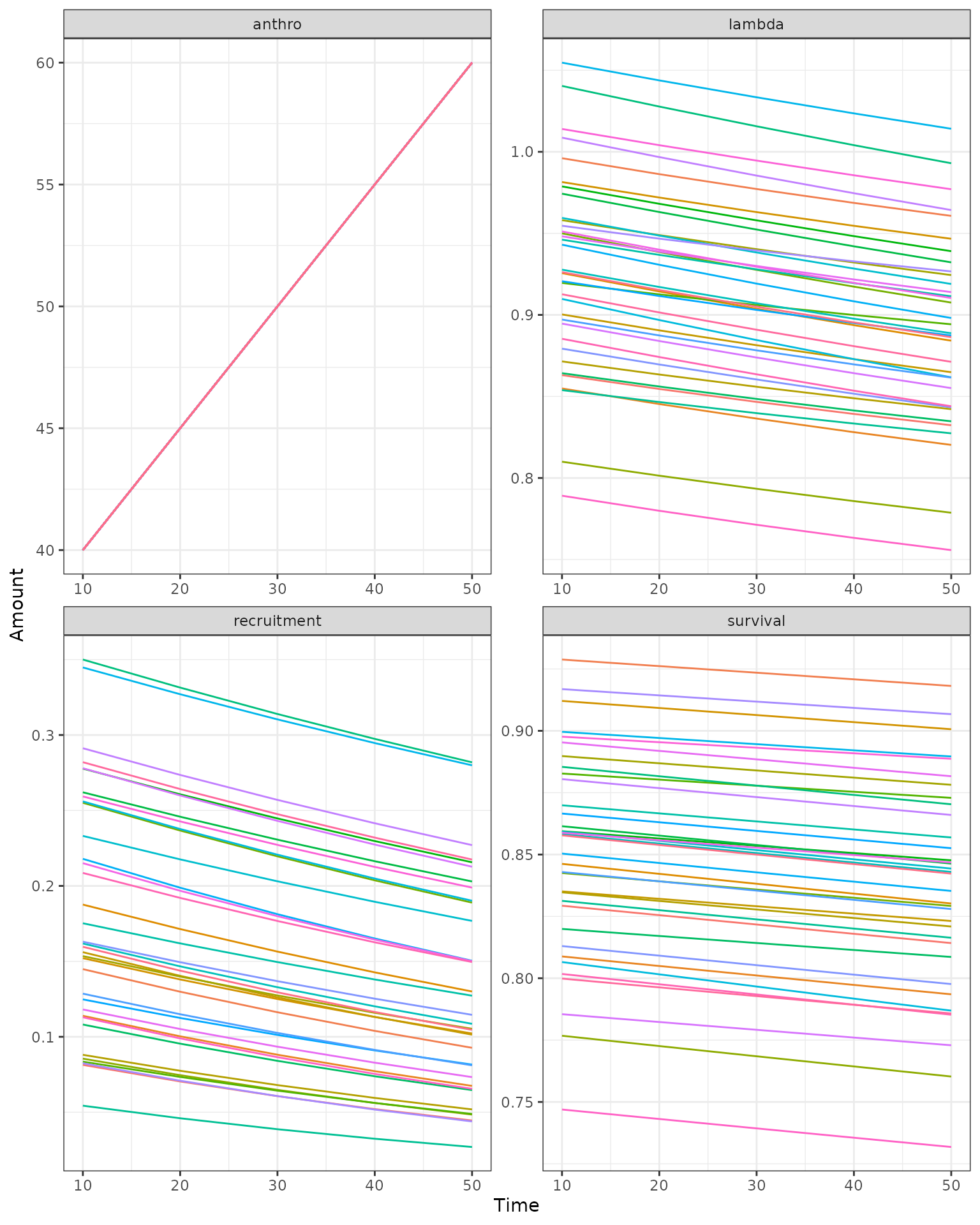

Figure 1.5: Example demographic trajectories from the national model on a changing landscape. ‘lambda’ is realized population growth rate in the final year, and ‘lambdaE’ is expected population growth rate without interannual variation, density dependence or demographic stochasticity. ‘N’ is the number of adult females. ‘R_bar/S_bar’ are the expected recruitment (calf:cow ratio) and survival rates, ‘R_t/S_t’ are the recruitment and survival rates.

1.5 Using the trajectoriesFromNational wrapper function to project population growth

The examples above show steps in the demographic modeling workflow. We also provide a trajectoriesFromNational wrapper function that samples the coefficients from the National model, calculates demographic rates given those coefficients and the level of disturbance, projects population growth using caribouPopGrowth, and returns summaries of the demographic rates (ref workflow diagram). If the disturbance scenario includes a Year column trajectoriesFromNational projects population growth over time, and also returns sample demographic trajectories. If year is not provided, population growth is projected for one year, and sample trajectories are not returned.

natTraj <- trajectoriesFromNational(replicates = 500, 
                                    disturbance = covTableSim, interannualVar = FALSE, 
                                    useQuantiles = TRUE)

# add year to return samples
natTraj35 <- trajectoriesFromNational(replicates = 35, 
                                    disturbance = covTableSim %>% 
                                      mutate(Year = Anthro+100*Fire_excl_anthro), 
                                    returnSamples = TRUE, interannualVar = FALSE, 
                                    useQuantiles = TRUE)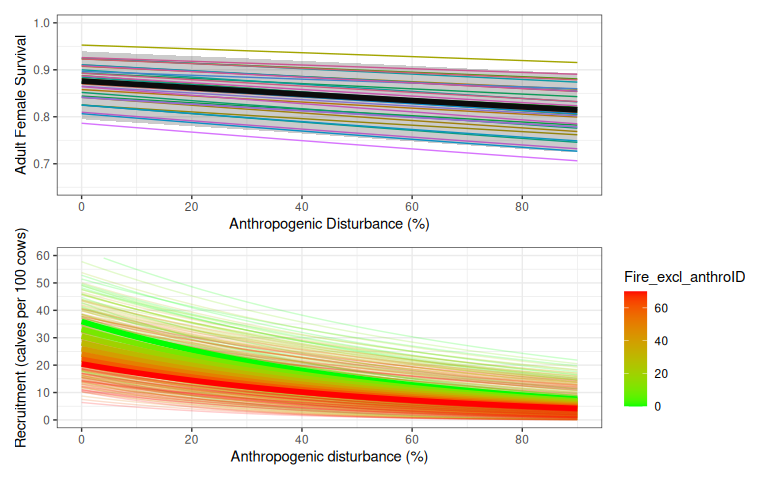

Figure 1.6: Variation in expected survival and recruitment with disturbance, obtained using the trajectoriesFromNational wrapper function. See Figure 1.3 for details.

Using the same scenario with anthropogenic disturbance footprint increasing by 5% per decade, we can also produce projections over a changing landscape with trajectoriesFromNational.

disturbance2 = data.frame(step = 0:40) %>% bind_cols(disturbance) %>% 
  mutate(Anthro = Anthro + AnthroChange * step, 
         Year = step)

# set seed so vignette looks the same each time
set.seed(123)

popMetrics2 <- trajectoriesFromNational(disturbance = disturbance2, replicates = 500, 
                                        useQuantiles = TRUE,N0 = 100, numSteps = 1)

popMetrics2$summary <- popMetrics2$summary %>% 
  filter(MetricTypeID %in% c("Anthro", "N", "Sbar","survival","Rbar","recruitment", "lambda_bar", "lambda"))
names <- popMetrics2$summary %>% select(MetricTypeID,Parameter) %>% unique()
popMetrics2$samples <- merge(popMetrics2$samples,names) %>%
  filter(as.numeric(as.factor(Replicate))<=35)

proj <- ggplot(data = popMetrics2$summary,
               aes(x=Year,y=Mean,ymin=lower,ymax=upper))+
  geom_ribbon(fill="grey") +
  geom_line(colour="black",linewidth=2)+
  geom_line(data=popMetrics2$samples,
            aes(x=Year,y=Amount,colour=Replicate, group=Replicate),
            inherit.aes = FALSE) +
  facet_wrap(~Parameter, scales = "free") +
  ylab("")+
  theme(legend.position = "none")

proj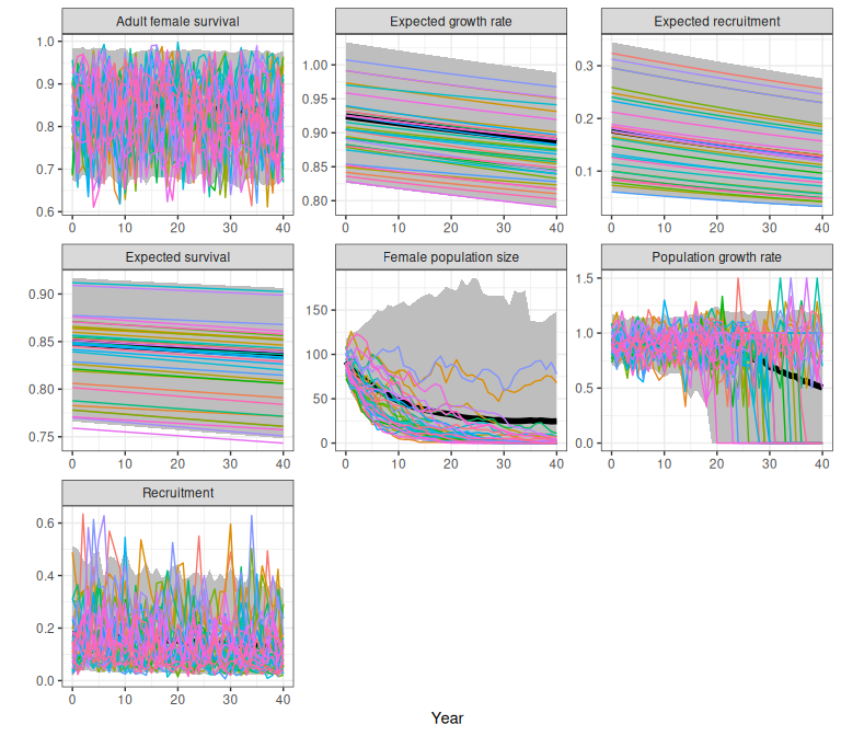

Figure 1.7: Example demographic trajectories and from the national model on a changing landscape, obtained using the trajectoriesFromNational wrapper function. Bands are the 2.5% and 97.5% quantiles of 500 samples. Female population size is shown separately with a log scaled y axis to allow comparison of divergent trajectories.

2 Demographic rates and trajectories from Bayesian models

2.1 Getting a fitted bboutools logistic model

See Comparing caribouMetrics (Beta) and bboutools (logistic) Bayesian models vignette for an overview of the Bayesian models. For this example we use a bboutools logistic model and example data.

library(bboudata)
library(bboutools)
useSaved <- T # option to skip slow step of fitting bboutools model
bbouInformativeFile <- here::here("results/vignetteBbbouExample.rds")
surv_data <- bboudata::bbousurv_a %>% filter(Year > 2010)
surv_data_add <- expand.grid(Year = seq(2017, 2022), Month = seq(1:12),
                             PopulationName = unique(surv_data$PopulationName))
surv_data <- merge(surv_data, surv_data_add, all.x = TRUE, all.y = TRUE)
recruit_data <- bboudata::bbourecruit_a %>% filter(Year > 2010)
recruit_data_add <- expand.grid(Year = seq(2017, 2022), PopulationName = unique(recruit_data$PopulationName))
recruit_data <- merge(recruit_data, recruit_data_add, all.x = TRUE, all.y = TRUE)
if (useSaved & file.exists(bbouInformativeFile)) {
  bbouInformative <- readRDS(bbouInformativeFile)
} else {
  bbouInformative <- estimateBayesianRates(surv_data, recruit_data,
                                          return_mcmc = TRUE)
  if (dir.exists(dirname(bbouInformativeFile))) {
    saveRDS(bbouInformative, bbouInformativeFile)
  }
}

2.2 Using bboutools to project population growth

The bboutools R package includes methods for projecting calf:cow ratios, recruitment, survival, and population growth rate. Note there is no population size, demographic stochasticity or density dependence in these projections.

predict_calfcow <- bboutools::bb_predict_calf_cow_ratio(bbouInformative$recruit_fit, year = TRUE)
bboutools::bb_plot_year_calf_cow_ratio(predict_calfcow)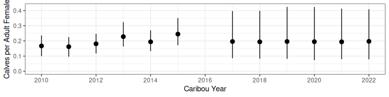

Figure 2.1: Calf:cow ratio projection from bboutools.

predict_recruitment <- bboutools::bb_predict_recruitment(bbouInformative$recruit_fit, year = TRUE)
bboutools::bb_plot_year_recruitment(predict_recruitment)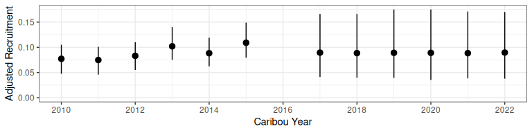

Figure 2.2: Recruitment projection from bboutools.

predict_survival <- bboutools::bb_predict_survival(bbouInformative$surv_fit, year = TRUE, month = FALSE)
bboutools::bb_plot_year_survival(predict_survival)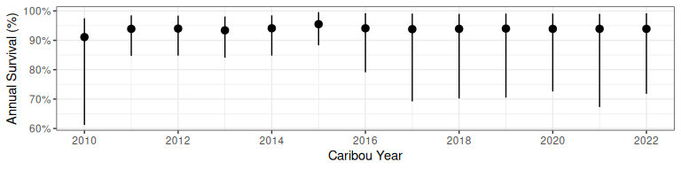

Figure 2.3: Survival projection from bboutools.

predict_lambda <- bboutools::bb_predict_growth(survival = bbouInformative$surv_fit, recruitment = bbouInformative$recruit_fit)
bboutools::bb_plot_year_growth(predict_lambda) +
  ggplot2::scale_y_continuous(labels = scales::percent)+
  ggplot2::ylab("Population growth rate")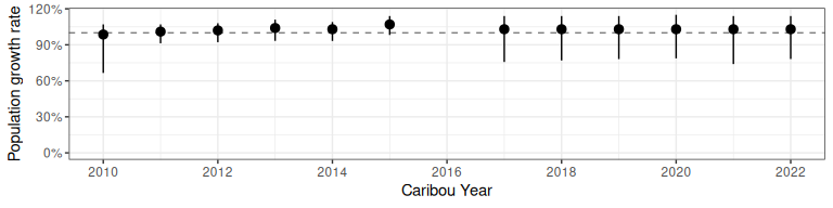

Figure 2.4: Population growth rate from bboutools.

2.3 Using the trajectoriesFromBayesian wrapper function to project population growth

For convenience, to enable comparisons (e.g. Comparing caribouMetrics (Beta) and bboutools (logistic) Bayesian models vignette), and to integrate with other methods and workflows, we can use the trajectoriesFromBayesian wrapper function to get sample trajectories and summaries from our fitted bboutools model. Note that if we use only the information in the fitted model (that does not include initial population size) then the summary results (bands for Adult female survival, Recruitment and Population growth rate in Figure 2.5) are identical to the bboutools projections (Figures 2.1, 2.3, and 2.4). The returned example trajectories are derived from the MCMC samples. If we also provide initial population size information then the projection (by default) includes density dependence and demographic stochasticity (Dyson et al. 2026; Hughes et al. 2025) and populations can go extinct (Fig 2.6). Note that in this case the form of the growth model (density dependence & demographic stochasticity, but not interannual variability) can be changed by setting caribouPopGrowth function parameters. The Bayesian MCMC samples include interannual variation in recruitment and survival, so no additional interannual variation is added by caribouPopGrowth in this case.

popMetricsBayes <- trajectoriesFromBayesian(bbouInformative)
popMetricsBayes$summary <- popMetricsBayes$summary %>% 
  filter(MetricTypeID %in% c("Sbar","survival","Rbar","recruitment", "lambda_bar", "lambda"))
names <- popMetricsBayes$summary %>% select(MetricTypeID,Parameter) %>% unique()
names
#>    MetricTypeID              Parameter
#> 1        lambda Population growth rate
#> 13   lambda_bar   Expected growth rate
#> 25         Rbar   Expected recruitment
#> 37  recruitment            Recruitment
#> 49         Sbar      Expected survival
#> 61     survival  Adult female survival

popMetricsBayes$samples <- popMetricsBayes$samples %>% 
  filter(MetricTypeID %in% c("Sbar","survival","Rbar",
                             "recruitment", "lambda_bar", "lambda")) %>% 
  merge(names) %>% 
  filter(as.numeric(as.factor(Replicate))<=35)

proj <- ggplot(data = popMetricsBayes$summary,
               aes(x=Year,y=Mean,ymin=lower,ymax=upper))+
  geom_ribbon(fill="grey") +
  geom_line(colour="black",linewidth=2)+
  geom_line(data=popMetricsBayes$samples,
            aes(x=Year,y=Amount,colour=Replicate,group=Replicate), inherit.aes = FALSE) +
  facet_wrap(~Parameter, scales = "free") +
  ylab("")+
  theme(legend.position = "none")
proj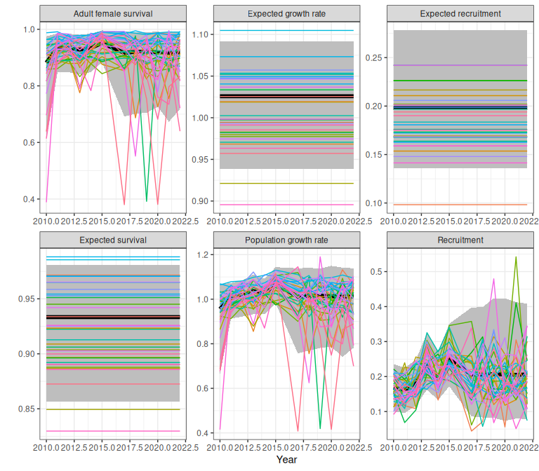

Figure 2.5: Example demographic trajectories from a fitted bboutools model, obtained using the trajectoriesFromBayesian wrapper function. Bands are 95% predictive intervals.

popMetricsBayes <- trajectoriesFromBayesian(bbouInformative,N0=100)
popMetricsBayes$summary <- popMetricsBayes$summary %>% 
  filter(MetricTypeID %in% c("survival","recruitment", "lambda_bar", "lambda","N"))
names <- popMetricsBayes$summary %>% select(MetricTypeID,Parameter) %>% unique()
names
#>    MetricTypeID              Parameter
#> 1        lambda Population growth rate
#> 13   lambda_bar   Expected growth rate
#> 25            N Female population size
#> 37  recruitment            Recruitment
#> 49     survival  Adult female survival

popMetricsBayes$samples <- popMetricsBayes$samples %>% 
  filter(MetricTypeID %in% c("survival","recruitment", "lambda_bar", "lambda","N")) %>% 
  merge(names) %>% 
  filter(as.numeric(as.factor(Replicate))<=35)

proj <- ggplot(data = popMetricsBayes$summary,
               aes(x=Year,y=Mean,ymin=lower,ymax=upper))+
  geom_ribbon(fill="grey") +
  geom_line(colour="black",linewidth=2)+
  geom_line(data=popMetricsBayes$samples,
            aes(x=Year,y=Amount,colour=Replicate,group=Replicate), inherit.aes = FALSE) +
  facet_wrap(~Parameter, scales = "free") +
  ylab("")+
  theme(legend.position = "none")
proj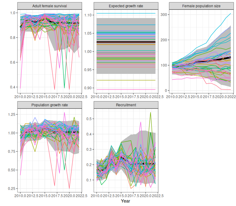

Figure 2.6: Example demographic trajectories from a fitted bboutools model, obtained using the trajectoriesFromBayesian wrapper function, with initial population size of 100. Bands are 95% predictive intervals.

2.4 Using the trajectoriesFromSummaries wrapper function to project population growth

To allow for the possibility of using fitted Bayesian models as a starting point for exploring demographic scenarios, the estimateBayesianRates function also returns a list of model parameters. The trajectoriesFromSummary projects outcomes from a model defined by these parameters. When parameters from a fitted Bayesian model are used, expected outcomes from trajectoriesFromSummary and trajectoriesFromBayesian are the same (Figure 2.7), but trajectoriesFromSummary projections do not include variation in interannual variation over time (Figure 2.8). trajectoriesFromSummary allows us to explore the implications of changing model parameters (Fig 2.9).

pt <- bbouInformative$parList
trajFromSummaryBase <- trajectoriesFromSummary(replicates=1000,N0=100,Rbar=pt$Rbar,
                                               Sbar=pt$Sbar, Riv=pt$Riv,Siv=pt$Siv,
                                               type=pt$type)
#> Compiling model graph
#>    Resolving undeclared variables
#>    Allocating nodes
#> Graph information:
#>    Observed stochastic nodes: 0
#>    Unobserved stochastic nodes: 14
#>    Total graph size: 111
#> 
#> Initializing model
#> 
#> Compiling model graph
#>    Resolving undeclared variables
#>    Allocating nodes
#> Graph information:
#>    Observed stochastic nodes: 0
#>    Unobserved stochastic nodes: 14
#>    Total graph size: 111
#> 
#> Initializing model
out_tbls <- compareTrajectories(trajFromSummaryBase, simInitial = popMetricsBayes)
typeLabs <- c("Summary", "Bayes")

recE <- plotCompareTrajectories(out_tbls, "Expected recruitment", typeLabels = typeLabs)
survE <- plotCompareTrajectories(out_tbls, "Expected survival", typeLabels = typeLabs)
lamE <- plotCompareTrajectories(out_tbls, "Expected growth rate", typeLabels = typeLabs,
                               lowBound = 0.5, highBound = 1.5)
recE /survE / lamE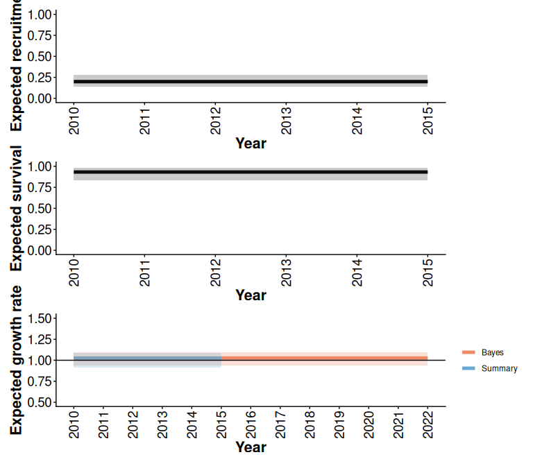

Figure 2.7: Comparison of expected demographic projections obtained using the trajectoriesFromSummary (Summary) and trajectoriesFromBayesian (Bayes) wrapper functions. Bands are the 2.5% and 97.5% quantiles of 500 samples.

rec <- plotCompareTrajectories(out_tbls, "Recruitment", typeLabels = typeLabs)
surv <- plotCompareTrajectories(out_tbls, "Adult female survival", typeLabels = typeLabs)
lam <- plotCompareTrajectories(out_tbls, "Population growth rate", typeLabels = typeLabs,
                               lowBound = 0.5, highBound = 1.5)
N <- plotCompareTrajectories(out_tbls, "Female population size", typeLabels = typeLabs,
                             lowBound = 0, highBound = 500)
rec /surv / lam / N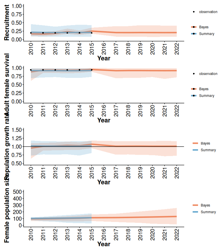

Figure 2.8: Comparison of demographic projections obtained using the trajectoriesFromSummary (Summary) and trajectoriesFromBayesian (Bayes) wrapper functions. Bands are the 2.5% and 97.5% quantiles of 500 samples.

pm.startYear <- 2015; pm.endYear <- 2022
RbarAdjust <- pt$Rbar
RbarAdjust$adjust.mu <- 0.1; RbarAdjust$adjust.sd <- 0.01
RbarAdjust$adjust.mu[(RbarAdjust$Year<pm.startYear)|(RbarAdjust$Year>=pm.endYear)]=0
RbarAdjust$adjust.sd[(RbarAdjust$Year<pm.startYear)|(RbarAdjust$Year>=pm.endYear)]=0
NAdjust <- data.frame(PopulationName <- unique(RbarAdjust$PopulationName))
NAdjust$N0 <- 100
NAdjust$N.sd <- 0.3*NAdjust$N0
NAdjust$N.lower <- 50
NAdjust$N.upper <- 200
trajFromSummaryAdjust <- trajectoriesFromSummary(replicates=1000,N0=NAdjust,Rbar=RbarAdjust,
                                               Sbar=pt$Sbar,
                                               Riv=pt$Riv,Siv=pt$Siv,
                                               type=pt$type)
#> Compiling model graph
#>    Resolving undeclared variables
#>    Allocating nodes
#> Graph information:
#>    Observed stochastic nodes: 0
#>    Unobserved stochastic nodes: 14
#>    Total graph size: 111
#> 
#> Initializing model
#> 
#> Compiling model graph
#>    Resolving undeclared variables
#>    Allocating nodes
#> Graph information:
#>    Observed stochastic nodes: 0
#>    Unobserved stochastic nodes: 14
#>    Total graph size: 117
#> 
#> Initializing model
out_tbls <- compareTrajectories(trajFromSummaryAdjust, simInitial = trajFromSummaryBase)
typeLabs <- c("Adjust", "Base")

rec <- plotCompareTrajectories(out_tbls, "Recruitment", typeLabels = typeLabs)
surv <- plotCompareTrajectories(out_tbls, "Adult female survival", typeLabels = typeLabs)
lam <- plotCompareTrajectories(out_tbls, "Population growth rate", typeLabels = typeLabs,
                               lowBound = 0.5, highBound = 1.5)
N <- plotCompareTrajectories(out_tbls, "Female population size", typeLabels = typeLabs,
                             lowBound = 0, highBound = 700)
rec /surv / lam / N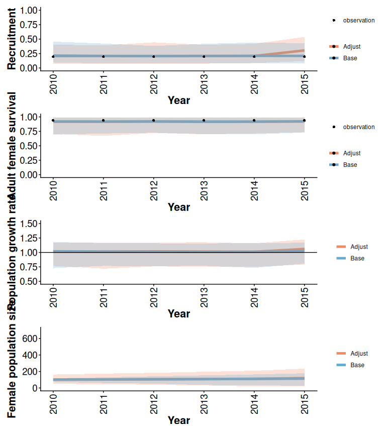

Figure 2.9: Effects of increasing recruitment after 2015 and increasing variation in initial population size on demographic projections obtained using the trajectoriesFromSummary wrapper function. Bands are the 2.5% and 97.5% quantiles of 500 samples.

2.5 Using the trajectoriesFromSummariesForApp wrapper function to project population growth

The trajectoriesFromSummaryForApp wrapper function is less flexible than trajectoriesFromSummary, and does not allow changes in demographic rates over time. It is used to enable scenario exploration in our Boreal Caribou Demographic Projection Explorer.

pt <- bbouInformative$parTab;pt
#>   PopulationName     R_bar     R_sd R_iv_mean R_iv_shape R_bar_lower
#> 1              A 0.1957146 0.223214 0.3769658   2.237384   0.1357969
#>   R_bar_upper     S_bar      S_sd S_iv_mean S_iv_shape S_bar_lower S_bar_upper
#> 1   0.2780221 0.9404699 0.5481804 0.5339908   1.141895   0.8566462   0.9804958
#>   N0 nCollarYears nSurvYears nCowsAllYears nRecruitYears
#> 1 NA           NA         12            NA            12

popMetricsBase <- trajectoriesFromSummaryForApp(numSteps=10,replicates=500,N0=500,R_bar=pt$R_bar,S_bar=pt$S_bar,
                                             R_sd=pt$R_sd,S_sd=pt$S_sd,
                                             R_iv_mean=pt$R_iv_mean,R_iv_shape=pt$R_iv_shape,
                                             S_iv_mean=pt$S_iv_mean,S_iv_shape=pt$S_iv_shape,
                                             scn_nm="base",doSummary=T)
popMetricsS85 <- trajectoriesFromSummaryForApp(numSteps=10,replicates=500,N0=500,R_bar=pt$R_bar,S_bar=0.85,
                                             R_sd=pt$R_sd,S_sd=pt$S_sd,
                                             R_iv_mean=pt$R_iv_mean,R_iv_shape=pt$R_iv_shape,
                                             S_iv_mean=pt$S_iv_mean,S_iv_shape=pt$S_iv_shape,
                                             scn_nm="S85",doSummary=T)
scnCompare <- list(summary=rbind(popMetricsBase$summary,popMetricsS85$summary),
                   samples=rbind(popMetricsBase$samples,popMetricsS85$samples))
scnCompare$summary <- scnCompare$summary %>% 
  filter(MetricTypeID %in% c("Anthro", "N", "Sbar","survival","Rbar","recruitment", "lambda_bar", "lambda"))
names <- scnCompare$summary %>% select(MetricTypeID,Parameter) %>% unique();names
#>    MetricTypeID              Parameter
#> 1        lambda Population growth rate
#> 11   lambda_bar   Expected growth rate
#> 21            N Female population size
#> 31  recruitment            Recruitment
#> 41     survival  Adult female survival
scnCompare$samples <- merge(scnCompare$samples,names) %>% filter(as.numeric(as.factor(Replicate))<=25)

proj <- ggplot(data = scnCompare$summary,
               aes(x=Year,y=Mean,ymin=lower,ymax=upper,fill=PopulationName,group=PopulationName))+
  geom_ribbon(alpha=0.2) +
  geom_line(linewidth=2,colour="black")+
  geom_line(data=scnCompare$samples,aes(x=Year,y=Amount,colour=PopulationName,group=paste0(Replicate,PopulationName),ymin=Amount,ymax=Amount)) +
  facet_wrap(~Parameter, scales = "free") +
  ylab("")
proj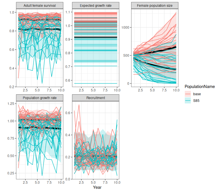

Figure 2.10: Comparison of demographic trajectories from a fitted bboutools model (base) and a scenario in which expected survival is increased to 85% (S85), obtained using the trajectoriesFromSummary wrapper function. Bands are the 2.5% and 97.5% quantiles of 500 samples.

References

Dyson, Matt, Sarah Endicott, Craig Simpkins, Julie W. Turner, Stephanie Avery-Gomm, Cheryl A. Johnson, Mathieu Leblond, et al. 2026. “Effective Conservation Decisions Require Models Designed for Purpose: A Case Study of Boreal Caribou in Ontario’s Ring of Fire.” Ecology and Evolution In press. https://doi.org/10.1101/2022.06.01.494350.

Ferrari, Silvia, and Francisco Cribari-Neto. 2004. “Beta Regression for Modelling Rates and Proportions.” Journal of Applied Statistics 31 (7): 799–815. https://doi.org/10.1080/0266476042000214501.

Hughes, Josie, Sarah Endicott, Anna M. Calvert, and Cheryl A. Johnson. 2025. “Integration of National Demographic-Disturbance Relationships and Local Data Can Improve Caribou Population Viability Projections and Inform Monitoring Decisions.” Ecological Informatics 87 (July): 103095. https://doi.org/10.1016/j.ecoinf.2025.103095.

Johnson, Cheryl A., Glenn D. Sutherland, Erin Neave, Mathieu Leblond, Patrick Kirby, Clara Superbie, and Philip D. McLoughlin. 2020. “Science to Inform Policy: Linking Population Dynamics to Habitat for a Threatened Species in Canada.” Journal of Applied Ecology 57 (7): 1314–27. https://doi.org/10.1111/1365-2664.13637.