Plot and compare Bayesian population model results

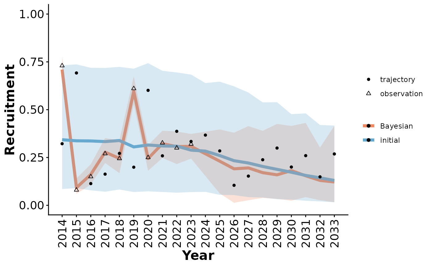
Plot Bayesian population model results, with (optionally) the distribution of outcomes from the initial model, local observations, and true local state for comparison.

Usage

plotCompareTrajectories(
  modTables,
  metric,
  lowBound = 0,
  highBound = 1,
  facetVars = NULL,
  labFontSize = 14,
  legendPosition = "right",
  breakInterval = 1,
  typeLabels = c("Bayesian", "initial")
)

Arguments

modTables

list. A list of model results tables created using [compareTrajectories()].

metric

character. Which metric to plot, if more than one, a list of plots is returned.

lowBound, highBound

numeric. Lower and upper y axis limits

facetVars

character. Optional. Vector of column names to facet by

labFontSize

numeric. Optional. Label font size if there are not facets. Font size is 10 pt if facets are used.

legendPosition

"bottom", "right", "left","top", or "none". Legend position.

breakInterval

number. How many years between x tick marks?

typeLabels

vector of two labels. Default c("Bayesian","initial"). Names of models to be compared.

Value

a ggplot object or list of ggplot objects if a vector of metrics was given.

Details

plotCompareTrajectories and plotTrajectories both plot Bayesian population model results over time but plotCompareTrajectories can to show results of the whole [bayesianScenariosWorkflow()] including simulation of observations, model fit and comparison to an initial model. See [plotTrajectories()] the ability to show multiple sample trajectories from one model

See also

Caribou demography functions: bayesianScenariosWorkflow(), bayesianTrajectoryWorkflow(), betaNationalPriors(), caribouPopGrowth(), compareTrajectories(), compositionBiasCorrection(), convertTrajectories(), dataFromSheets(), demographicProjectionApp(), demographyDefaults(), disturbanceDefaults(), estimateBayesianRates(), estimateNationalRate(), getNationalCoefficients(), getScenarioDefaults(), monitoringDefaults(), nationalTrajectoryDefaults(), plotSurvivalSeries(), plotTrajectories(), popGrowthTableJohnsonECCC, simulateObservations(), timeDefaults(), trajectoriesFromBayesian(), trajectoriesFromNational(), trajectoriesFromSummary(), trajectoriesFromSummaryForApp()

Examples

scns <- getScenarioDefaults(projYears = 10, obsYears = 10,
                            obsAnthroSlope = 1, projAnthroSlope = 5,
                            collarCount = 20, cowMult = 5)

simO <- simulateObservations(scns)

out <- bayesianTrajectoryWorkflow(surv_data = simO$simSurvObs, recruit_data = simO$simRecruitObs,
                          disturbance = simO$simDisturbance,
                          startYear = 2014, niters=10)
#> Warning: requested year range: 2014 - 2033 does not match recruitment data year range:  2015 - 2025
#> Warning: missing years of recruitment data: 2014
#> Compiling model graph
#>    Resolving undeclared variables
#>    Allocating nodes
#> Graph information:
#>    Observed stochastic nodes: 10
#>    Unobserved stochastic nodes: 33
#>    Total graph size: 665
#> 
#> Initializing model
#> 
#> Warning: Adaptation incomplete
#> NOTE: Stopping adaptation
#> 
#> 
#> Compiling model graph
#>    Resolving undeclared variables
#>    Allocating nodes
#> Graph information:
#>    Observed stochastic nodes: 22
#>    Unobserved stochastic nodes: 77
#>    Total graph size: 694
#> 
#> Initializing model
#> 
#> Warning: Adaptation incomplete
#> NOTE: Stopping adaptation
#> 
#> 

out_tbl <- compareTrajectories(out, exData = simO$exData, paramTable = simO$paramTable,
                           simInitial = trajectoriesFromNational())
#> Using saved object

plotCompareTrajectories(out_tbl, metric = "Recruitment")