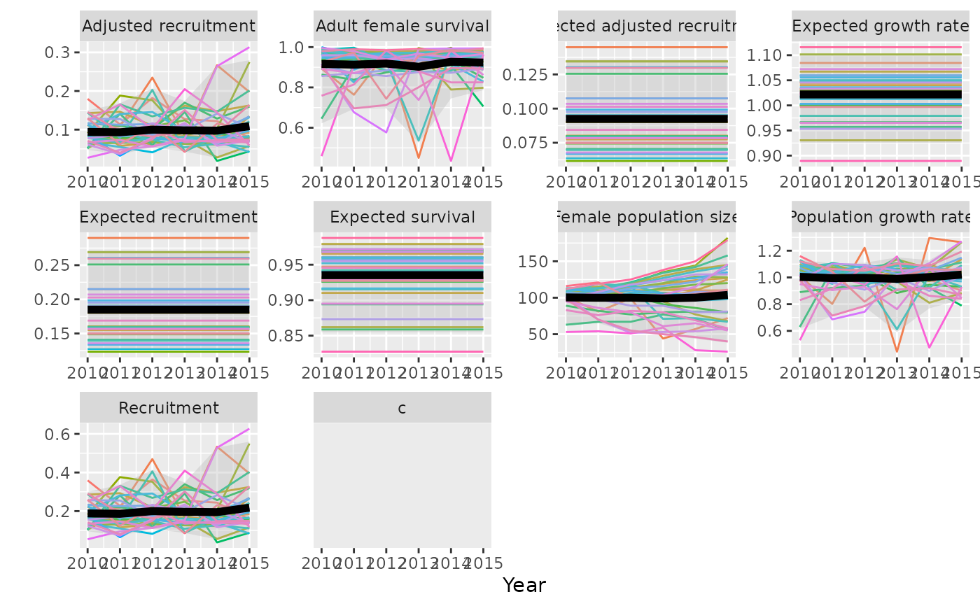
Plot Bayesian population model trajectories

Plot Bayesian population model results including multiple sample trajectories to show variation within the model. If results include multiple populations each population is shown with a different colour.

Usage

plotTrajectories(
  caribouBayesDemogMod,
  replicates = 35,
  metrics = c("Adult female survival", "Recruitment", "Adjusted recruitment",
    "Population growth rate", "Female population size", "c", "Expected survival",
    "Expected recruitment", "Expected adjusted recruitment", "Expected growth rate")
)

Arguments

caribouBayesDemogMod

list. Caribou Bayesian demographic model results produced by calling bayesianTrajectoryWorkflow(), trajectoriesFromNational(), trajectoriesFromBayesian(), or trajectoriesFromSummary().

replicates

integer. Number of replicate populations. Ignored if samples not included in caribouBayesDemogMod.

metrics

character. A vector of Metrics to be included as facets in the plot.

Details

plotTrajectories and plotCompareTrajectories both plot Bayesian population model results over time but plotTrajectories creates a faceted plot of several metrics with the ability to show sample trajectories along with the overall model prediction. See [plotCompareTrajectories] for displaying the results of [bayesianScenariosWorkflow()].

See also

Caribou demography functions: bayesianScenariosWorkflow(), bayesianTrajectoryWorkflow(), betaNationalPriors(), caribouPopGrowth(), compareTrajectories(), compositionBiasCorrection(), convertTrajectories(), dataFromSheets(), demographicProjectionApp(), demographyDefaults(), disturbanceDefaults(), estimateBayesianRates(), estimateNationalRate(), getNationalCoefficients(), getScenarioDefaults(), monitoringDefaults(), nationalTrajectoryDefaults(), plotCompareTrajectories(), plotSurvivalSeries(), popGrowthTableJohnsonECCC, simulateObservations(), timeDefaults(), trajectoriesFromBayesian(), trajectoriesFromNational(), trajectoriesFromSummary(), trajectoriesFromSummaryForApp()

Examples

# trajectories from arbitrary demographic rates

traj <- trajectoriesFromSummary(replicates = 35, N0 = 100,
                        Rbar = data.frame(mean = 0.19, sd = 0.23, lower = 0.13,
                                          upper = 0.27, Annual = 2010:2015, Year = 2010:2015,
                                          PopulationName = "A"),
                        Sbar = data.frame(mean = 0.94, sd = 0.61, lower = 0.86,
                                          upper = 0.98, Annual = 2010:2015, Year = 2010:2015,
                                          PopulationName = "A"),
                        Riv = data.frame(R_iv_mean = 0.36, R_iv_shape = 2),
                        Siv = data.frame(S_iv_mean = 0.63, S_iv_shape = 1.4),
                        type = "bbou")
#> Compiling model graph
#>    Resolving undeclared variables
#>    Allocating nodes
#> Graph information:
#>    Observed stochastic nodes: 0
#>    Unobserved stochastic nodes: 14
#>    Total graph size: 111
#> 
#> Initializing model
#> 
#> Compiling model graph
#>    Resolving undeclared variables
#>    Allocating nodes
#> Graph information:
#>    Observed stochastic nodes: 0
#>    Unobserved stochastic nodes: 14
#>    Total graph size: 111
#> 
#> Initializing model
#> 
plotTrajectories(traj)
#> Warning: Removed 210 rows containing missing values or values outside the scale range
#> (`geom_line()`).
#> Warning: Removed 6 rows containing missing values or values outside the scale range
#> (`geom_ribbon()`).
#> Warning: Removed 6 rows containing missing values or values outside the scale range
#> (`geom_line()`).