Introduction
This tutorial on using the projectRoads function of the
roads package to project forest road networks borrows
heavily from a demonstration written by Kyle Lochhead and Tyler Muhly in
2018. Example data sets used below are included in the package as
CLUSexample and demoScen.
There are three main inputs to the projectRoads
function:
-
weightRaster and weightFunction: together, these
determine the cost to build a road between two adjacent raster cells.
The
weightRasteris a spatial gridded raster with values for all locations where road construction is possible. TheweightFunctioncalculates the cost of constructing a road between two adjacent raster cells from theweightRasterat each of those cells. - Existing Road Network: a spatial representation of the existing road network.
- Landings: a set of locations to be connected to the existing road network by constructing new roads.
projectRoads simulates new roads that connect landings
to the existing road network using one of four methods:
- Snap
- Least-cost path (LCP)
- Iterative least-cost path (ILCP)
- Minimum spanning tree (MST)
The output of projectRoads is a list of simulation
results referred to as a “sim list”. The list contains five
elements:
- roads: the projected road network, including new and input roads.
-
weightRaster: the updated
weightRasterin which new and old roads have value 0. - roadMethod the road simulation method used.
- landings the landings used in the simulation.
-
g the graph that describes the cost of paths
between each cell in the updated
weightRaster. Edges between vertices connected by new roads have weight 0.gcan be used to avoid the cost of rebuilding the graph in a simulation with multiple time steps.
Setup
library(terra)
library(dplyr)
library(sf)
library(roads)

## colours for displaying weight raster
if(requireNamespace("viridis", quietly = TRUE)){
  # Use colour blind friendly palette if available
  rastColours <- c('grey50', viridis::viridis(20))
} else {
  rastColours <- c('grey50', terrain.colors(20))
}

# terra objects need to be wrapped to be saved, this unwraps them
CLUSexample <- prepExData(CLUSexample)
Resource development scenario
1. Weights Raster and Weight Function
The cost of constructing a road segment to connect adjacent cells is
determined by the weightFunction and the
weightRaster. The weightFunction calculates
the cost of construction between adjacent cells from the value of the
weightRaster at those cells and the distance between them.
Two methods of calculating costs are provided, and there is an option
for users to develop their own. The default
weightFunction = simpleCostFn assumes that the values in
the weightRaster represent the cost of building a road
across a cell, and sets cost as the mean value of adjacent cells. The
alternative weightFunction = gradePenaltyFn penalizes road
construction on steep grades by setting cost as a function of the
difference in weightRaster values between adjacent cells.
In this case, the weightRaster is an elevation raster that
can also include barriers. See ?gradePenaltyFn for
details.
The following points apply to all weightRasters:
- The
weightRastermust be a single, numericSpatRasterorRasterLayerobject. - The coordinate reference system (CRS) of this raster must match the
CRS of the existing road network and landings.
- The
weightRasterdetermines the extent of area considered for new road construction. Existing roads and landings outside the extent of theweightRasterare ignored. - Values of cells that include existing roads should be 0, and all 0
values are assumed to be existing roads. Existing roads can be added to
weightRasterby settingroadsInWeight = FALSE. - The resolution of the
weightRasterdetermines the resolution of the constructed road network. Adjacent cells are connected with straight road segments, and each cell either contains a road, or it does not. - NA values in the
weightRasterare not included in the graph, and are not considered for road construction. A landing surrounded by NAs that cannot be connected to the existing road network will produce an error.
The weight raster for this basic example is a cost surface and the
weightFunction used is the average.
weightRaster <- CLUSexample$cost2. Existing road network layer
The network of existing roads must be provided as an sf
object with geometry type "LINES", a
SpatialLines object, a RasterLayer, or a
SpatRaster. If the input roads are a raster the projected
roads will also be returned as a raster by default, but if
roadsOut = "sf" then a geometry collection of lines and
points will be returned with points representing the input roads.
The road network included in the CLUSexample data-set is
a raster but we use a line for plotting.
3. Landings layer(s)
Landings, or resource development locations, that are to be connected to the existing road network can be specified in a variety of forms:
- A
sfobject with geometry type"POINTS"or"POLYGON" - A logical
SpatRasterorRasterLayerobject with cell values ofTRUEfor landings, - A
SpatialPointsorSpatialPointsDataFrameobject with points representing landings, - A matrix with at least two columns, with columns 1 and 2 representing x any y coordinates of landing locations respectively,
- A
SpatialPolygonsorSpatialPolygonsDataFrameobject with polygons representing landings,
If the landings are polygons then the centroid is used as the destination for new roads. For more control or to specify more than one landing per polygon see Multiple landings per harvest section below.
## landings as spatial points
landings <- roads::CLUSexample$landings

## plot example scenario
par(omi = c(0,0,0,1.2))
plot(weightRaster, col = rastColours, main = 'Example Scenario')
plot(roadsLine, add = TRUE)
plot(landings, add = TRUE, pch = 19)
legend(x = 7.25, y = 5, legend = c("landings", "roads"), pch = c(19, NA),
       lwd = c(NA, 1),
       xpd = NA, inset = -0.1, xjust = 1)
Notice that the top row of the raster has a cost of zero where an existing road traverses the landscape.
Simulation of new roads development
Simulation methods
1. Snapping
This approach simply ‘snaps’ a landing to the nearest (by Euclidean distance) existing road segment, ignoring spatial variation in road construction cost and the locations of other landings and access roads.
## project new roads using the 'snap' approach
projRoads_snap <- roads::projectRoads(landings, weightRaster, roadsLine,
                                      roadMethod = 'snap')
#> 0s detected in weightRaster raster, these will be considered as existing roads

par(omi = c(0,0,0,1.2))
## plot the weight raster, landings, and roads segments to the landings
plot(weightRaster, col = rastColours, main = "'Snapped' roads")
points(landings, pch = 19)
plot(projRoads_snap$roads, add = TRUE)

## update legend
legend(x = 7.25, y = 5, legend = c("landings", "roads"), pch = c(19, NA),
       lwd = c(NA, 1),
       xpd = NA, inset = -0.1, xjust = 1)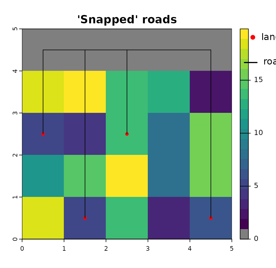
This simple approach gives an unrealistically redundant road network without branches that does not account for variation in road construction costs across the landscape.
2. Least Cost Paths (LCP)
The least cost paths method builds a ‘cost directed’ path (i.e., “as
the wolf runs”) for each landing to the existing road network. A
mathematical graph with a node
for each non-NA cell in the weightRaster and edge weights
determined by the weightFunction is built using igraph. The graph is used
to compute least cost paths between each landing and the nearest
existing road using Dijkstra’s
algorithm implemented in the shortest_paths
function in igraph. Graph weights are updated to include
new roads after all new roads are identified.
## project new roads using the 'LCP' approach
projRoads_lcp <- roads::projectRoads(landings,
                                        weightRaster,
                                        roadsLine,
                                        roadMethod = 'lcp')
#> 0s detected in weightRaster raster, these will be considered as existing roads

par(omi = c(0,0,0,1.2))
## plot the weight raster and overlay it with new roads
plot(weightRaster, col = rastColours, main = "'LCP' roads")
plot(projRoads_lcp$roads, add = TRUE)
points(landings, pch = 19)
## legend
legend(x = 7.25, y = 5, legend = c("landings", "roads"), pch = c(19, NA),
       lwd = c(NA, 1),
       xpd = NA, inset = -0.1, xjust = 1)
The main disadvantage of this approach is that roads are developed independently, which tends to produce parallel or redundant roads. This could mimic road development in cases where licensees restrict others from using their road (i.e., gated roads), and thereby force others to consider building a nearly parallel road. In some cases there will be branching, where two roads connecting two landings to an existing road network will use the same least cost path; however, this will be conditional on the spatial configuration of the local cost surface and the existing road network.
3. Iterative Least Cost Paths (ILCP)
This approach builds fewer redundant roads than the LCP method
because the graph edge weights are updated after each landing is
accessed, so that roads built earlier can be reused to access other
landings. The order is determined by the ordering argument
to projectRoads; by default the closest landings are
accessed first. The alternative ordering = none builds
roads in the order that landings are supplied by the user.
## project new roads using the 'ILCP' approach
projRoads_ilcp <- roads::projectRoads(landings,
                                        weightRaster,
                                        roadsLine,
                                        roadMethod = 'ilcp')
#> 0s detected in weightRaster raster, these will be considered as existing roads

par(omi = c(0,0,0,1.2))
## plot the weight raster and overlay it with new roads
plot(weightRaster, col = rastColours, main = "'ILCP' roads")
plot(projRoads_ilcp$roads, add = TRUE)
points(landings, pch = 19)  ## landings points
## legend
legend(x = 7.25, y = 5, legend = c("landings", "roads"), pch = c(19, NA),
       lwd = c(NA, 1),
       xpd = NA, inset = -0.1, xjust = 1)
The ILCP approach produces a more realistic branching network with less redundancy. However, it is sensitive to the ordering of the landings. Below we reverse the order of the landings but continue using the default ordering of closest first. The two closest landings are tied for distance to the road and the tie is broken by the order they are supplied in so switching that produces a different road network.
## project new roads using the 'ILCP' approach
projRoads_ilcp2 <- roads::projectRoads(st_coordinates(landings)[4:1,],
                                        weightRaster,
                                        roadsLine,
                                        roadMethod = 'ilcp')
#> 0s detected in weightRaster raster, these will be considered as existing roads
#> CRS of landings supplied as a matrix is assumed to match the weightRaster

par(omi = c(0,0,0,1.2))
## plot the weight raster and overlay it with new roads
plot(weightRaster, col = rastColours, main = "'ILCP' roads")
plot(projRoads_ilcp2$roads, add = TRUE)
points(landings, pch = 19)  ## landings points
## legend
legend(x = 7.25, y = 5, legend = c("landings", "roads"), pch = c(19, NA),
       lwd = c(NA, 1),
       xpd = NA, inset = -0.1, xjust = 1)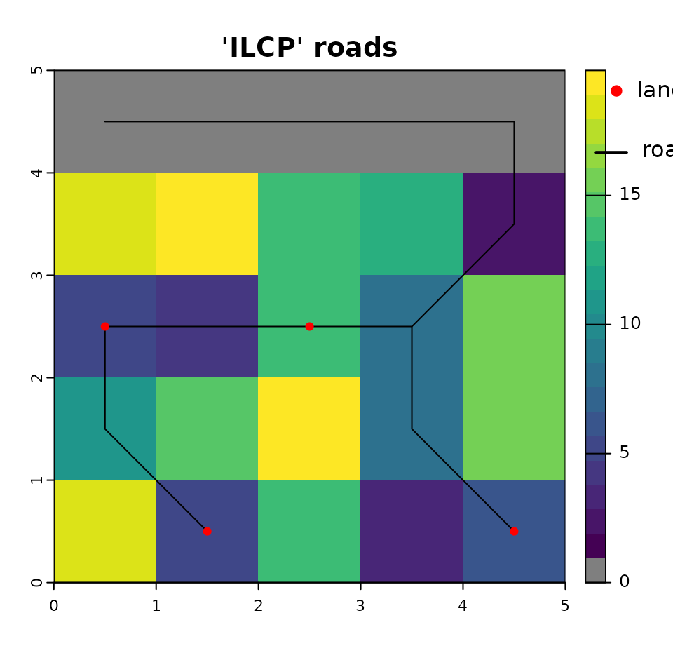
4. Minimum Spanning Tree (MST) with Least Cost Paths (LCP)
The MST approach builds upon the LCP approach by determining if landings should be connected to one another before being connected to the existing road network. In the MST approach, LCPs are estimated both between the landings and between landings and the existing road network. These distances are then used as nodes for solving a minimum spanning tree network that minimizes the overall cost of connecting all landings to the existing road network.
## project new roads using the 'MST' approach
projRoads_mst <- roads::projectRoads(landings,
                                        weightRaster,
                                        roadsLine,
                                        roadMethod = 'mst')
#> 0s detected in weightRaster raster, these will be considered as existing roads

par(omi = c(0,0,0,1.2))
## plot the weight raster and overlay it with new roads
plot(weightRaster, col = rastColours, main = "'MST' roads")
plot(projRoads_mst$roads, add = TRUE)
points(landings, pch = 19)
## legend
legend(x = 7.25, y = 5, legend = c("landings", "roads"), pch = c(19, NA),
       lwd = c(NA, 1),
       xpd = NA, inset = -0.1, xjust = 1)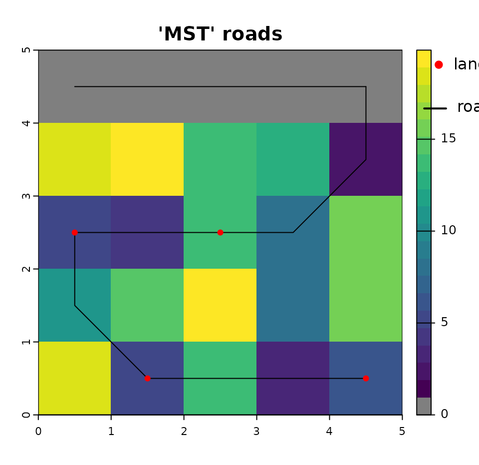
The MST approach will produce fewer roads than the other approaches, and realistic branching patterns. However, it is also more computationally costly than the other methods.
One-time versus multi-temporal simulation
Roads can be projected over a single time step (one-time) or over
multiple time steps. To demonstrate construction over multiple time
steps we use a demonstration scenario demoScen data-set
included in the roads package. The scenario includes four different sets
of landings.
## colours for displaying weight raster
if(requireNamespace("viridis", quietly = TRUE)){
  # Use colour blind friendly palette if available
  rastColours2 <- c('grey50', viridis::viridis(30))
} else {
  rastColours2 <- c('grey50', terrain.colors(30))
}

## scenario
demoScen <- prepExData(demoScen)
scen <- demoScen[[1]]
## landing sets 1 to 4 of this scenario
land.pnts <- scen$landings.points[scen$landings.points$set %in% c(1:4),]
## plot the weight raster and landings
par(mar=par('mar')/2)
plot(scen$cost.rast, col = rastColours2, main = 'Cost and landings (by set)')
plot(land.pnts %>% st_geometry(), add = TRUE, pch = 21, cex = 2, bg = 'white')
text(st_coordinates(land.pnts), labels = land.pnts$set, cex = 0.6, adj = c(0.5, 0.3),
     xpd = TRUE)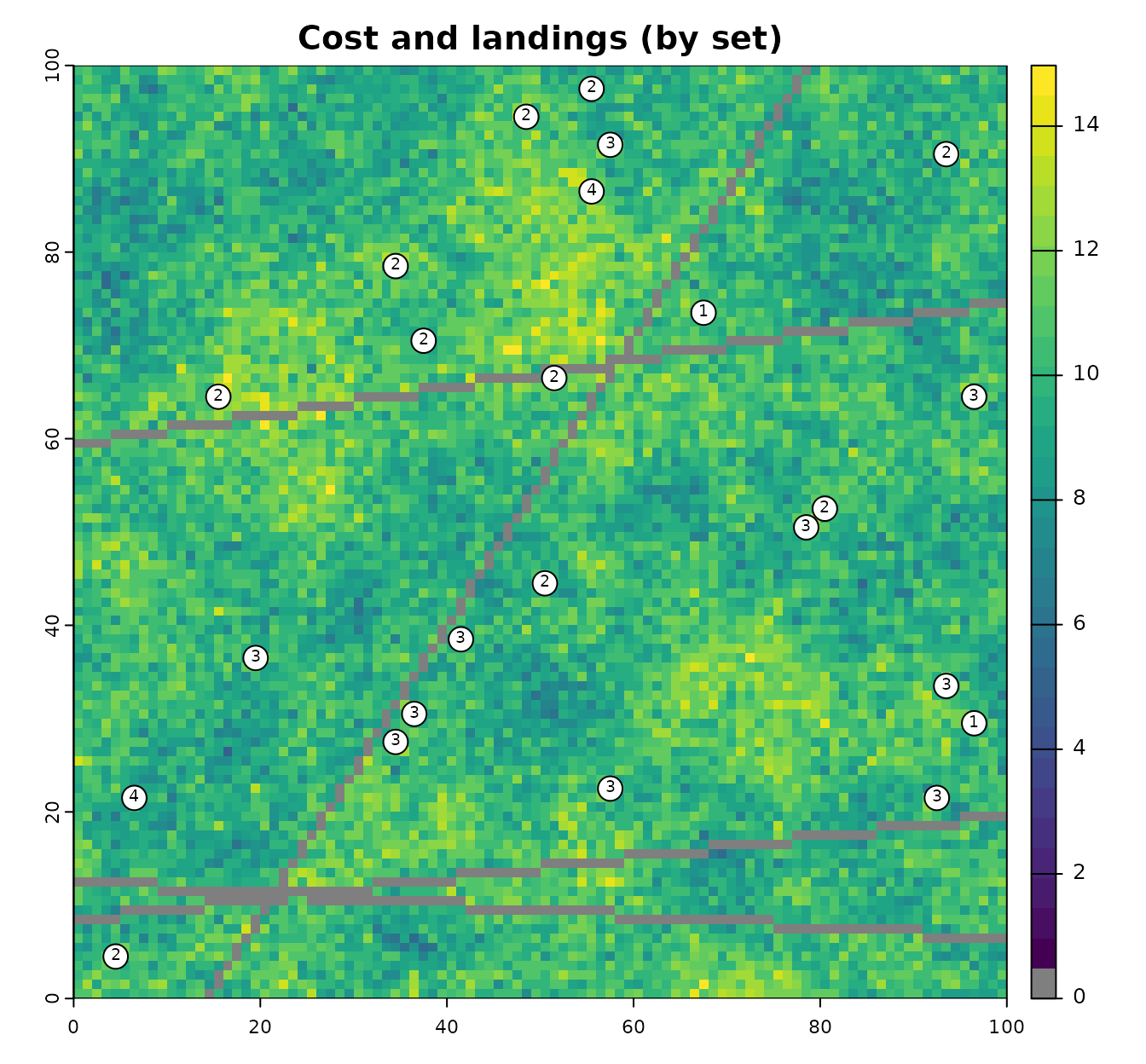
One-time simulation
If landings, costs, and roads are all specified to
projectRoads, then a one-time road simulation will be
performed that returns a list object holding the projected roads and
related information. This can be repeated multiple times for different
road building scenarios but each simulation will be independent of the
others.
## project roads for landing sets 1 to 4, with independent one-time simulations
oneTime_sim <- list() ## empty list
for (i in 1:4){
  oneTime_sim <- c(oneTime_sim,
                       roads::projectRoads(land.pnts[land.pnts$set==i,],
                                              scen$cost.rast,
                                              scen$cost.rast==0,
                                              roadMethod='mst')$roads)
}
#> 0s detected in weightRaster raster, these will be considered as existing roads
#> 0s detected in weightRaster raster, these will be considered as existing roads
#> 0s detected in weightRaster raster, these will be considered as existing roads
#> 0s detected in weightRaster raster, these will be considered as existing roads

## plot
oldpar <- par(mfrow = c(2, 2), mar = par('mar')/2)
for (i in 1:4){
  oneTime_sim[[i]][!oneTime_sim[[i]]] <- NA
  plot(scen$cost.rast, col = rastColours2,
       main = paste0('Landings set ', i),
       legend = FALSE)
  plot(oneTime_sim[[i]], add = TRUE, col = "grey50", legend = FALSE)
  plot(st_geometry(land.pnts[land.pnts$set == i, ]), add = TRUE,
       pch = 21, cex = 1.5, bg = 'white')
}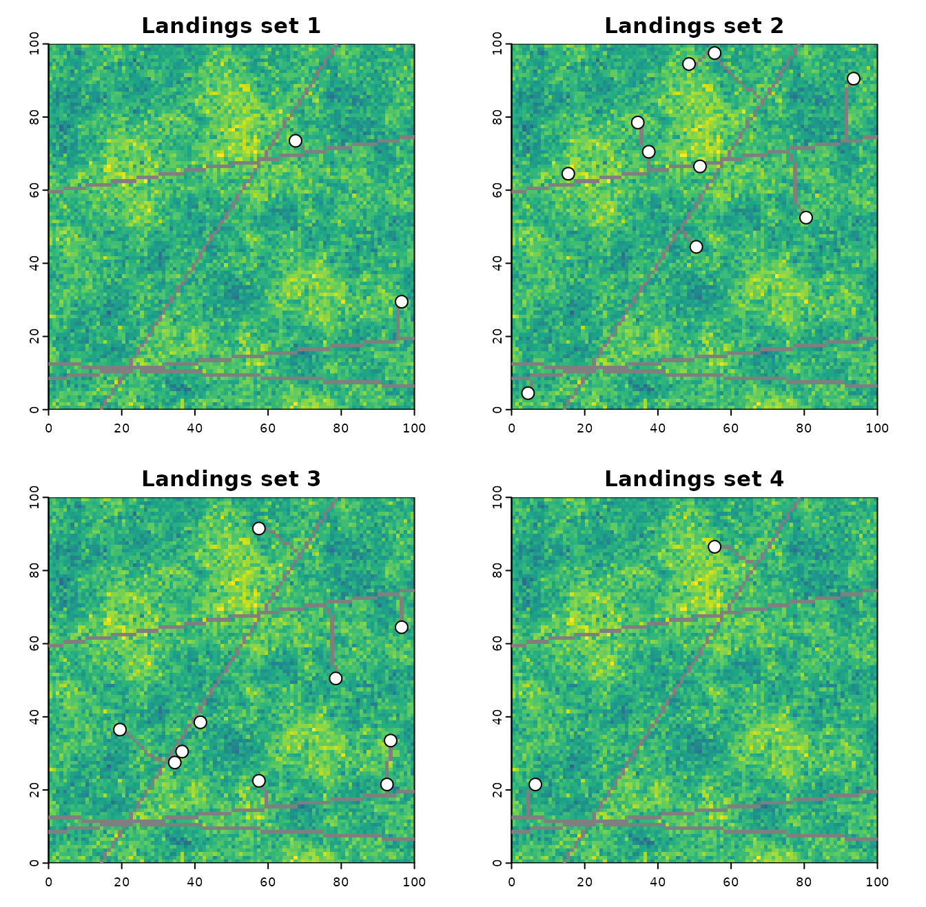
These independent one-time simulations are appropriate if each landing set represents a different development scenario (e.g. each representing a possible set of landings at time t=1), but they are not appropriate if landings sets are sequential (e.g. set 1 is development at time t=1, set 2 is development at time t=2, and so on). In the latter case, roads at the beginning of time t should be the union of roads developed in all previous times steps.
## raster representing the union of completely independent simulations for multiple sets
oneTime_sim <- rast(oneTime_sim)
independent <- any(oneTime_sim, na.rm = TRUE)
## set non-road to NA for display purposes
independent[!independent] <- NA

## plot
plot(scen$cost.rast, col = rastColours2,
     main = 'Union of independent sim results',
     legend = FALSE)

plot(independent, col = 'grey30', add = TRUE, legend = FALSE)

plot(st_geometry(land.pnts), add = TRUE, pch = 21, cex = 1.5, bg = 'white')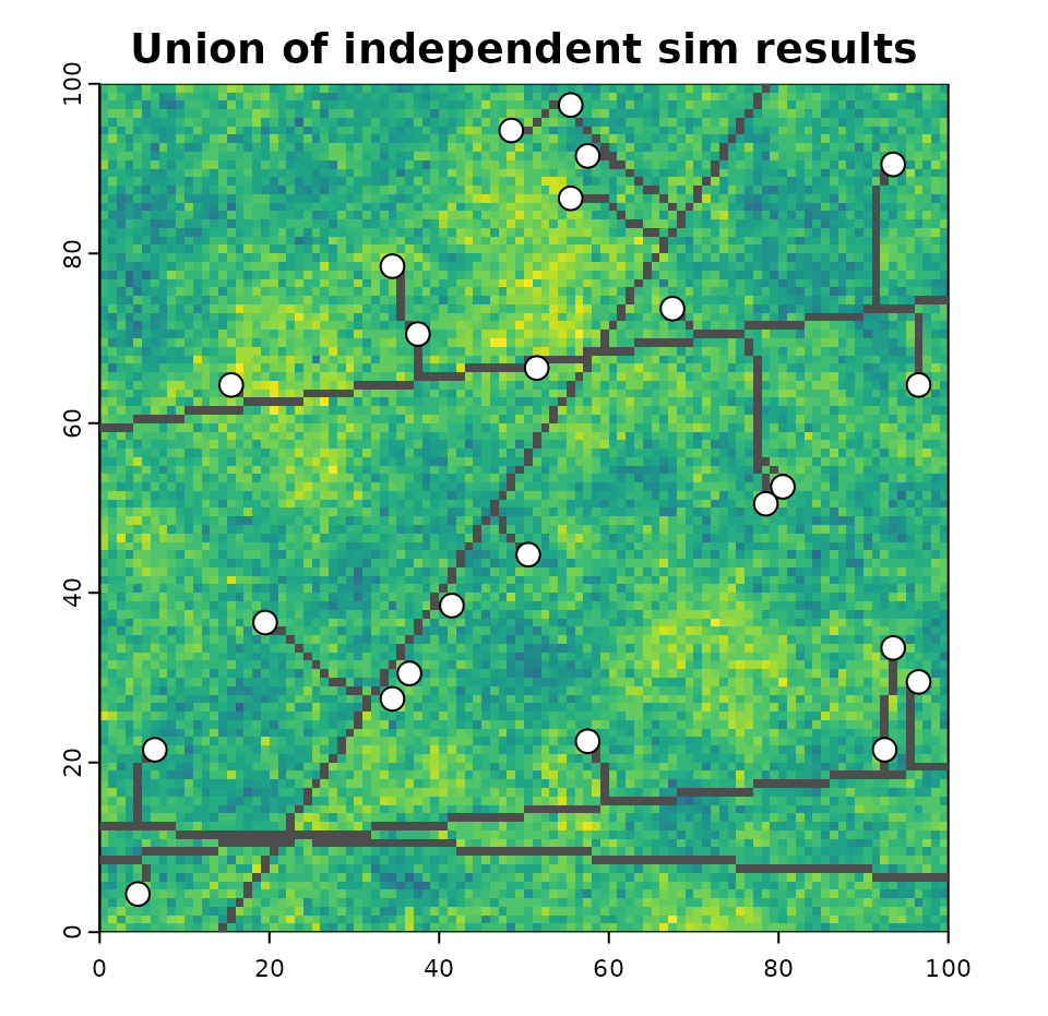
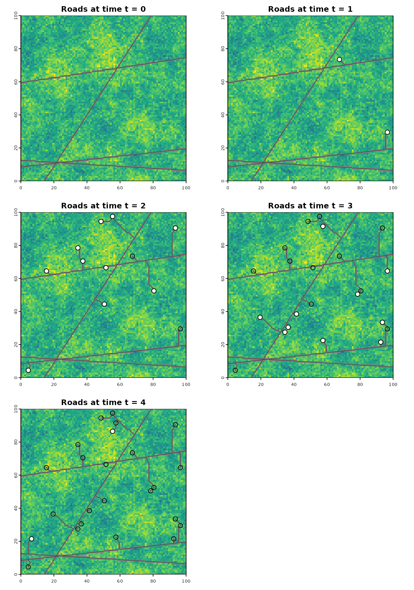
Multi-temporal simulation
Multi-temporal (multiple time steps) road projections can be obtained
by providing projectRoads with the list produced by a
previous call to projectRoads, and a new set of landings.
The function uses the sim list as a starting point, and
avoids the computational cost of reconstructing the landscape graph.
This can be implemented in a loop.
## continuing on with demo scenario 1
## landing sets 1 to 4 of this scenario as a raster stack
land.stack <- scen$landings.stack[[1:4]]

# initialize sim list with first landings set
multiTime_sim <- list(projectRoads(land.stack[[1]], scen$cost.rast,
                                               scen$road.line))
#> 0s detected in weightRaster raster, these will be considered as existing roads
#> harvest raster values are all in 0,1. Using patches as landing areas

# iterate over landings sets using the sim list from the previous run as input
for (i in 2:nlyr(land.stack)) {
  multiTime_sim <- c(
    multiTime_sim,
    list(projectRoads(sim =  multiTime_sim[[i-1]], landings = land.stack[[i]]))
  )
}
#> 0s detected in weightRaster raster, these will be considered as existing roads
#> harvest raster values are all in 0,1. Using patches as landing areas
#> 0s detected in weightRaster raster, these will be considered as existing roads
#> harvest raster values are all in 0,1. Using patches as landing areas
#> 0s detected in weightRaster raster, these will be considered as existing roads
#> harvest raster values are all in 0,1. Using patches as landing areas

par(mfrow = c(3, 2))
par(mar = par('mar')/2)
  plot(scen$cost.rast, col = rastColours2, main = 'Roads at time t = 0',
       legend = FALSE)
  plot(scen$road.line, col = 'grey30', add = TRUE, legend = FALSE)

for (i in 1:length(multiTime_sim)){
  plot(multiTime_sim[[i]]$weightRaster, col = rastColours2,
       main = paste0('Roads at time t = ', i), legend = FALSE)
  plot(multiTime_sim[[i]]$roads, col = 'grey30', add = TRUE, legend = FALSE)
  plot(st_geometry(land.pnts[land.pnts$set == i, ]), add = TRUE, pch = 21,
         cex = 1.5, bg = 'white')
  if (i >= 2){
    plot(st_geometry(land.pnts[land.pnts$set < i, ]), add = TRUE, pch = 1, cex = 1.5)
    plot(st_geometry(land.pnts[land.pnts$set == i, ]), add = TRUE, pch = 21,
         cex = 1.5, bg = 'white')
  }
}
Multiple landings per harvest block
Often harvest information is available as polygons showing the
cutover area but the point locations of landings are not known. The
roads package includes the getLandingsFromTarget function
to address these situations. By default
getLandingsFromTarget will use the centroid of a polygon as
the landing but other sampleType options include
"random" or "regular" selection of multiple
landing points within harvest blocks. For "random" or
"regular" sampling, landingDens specifies the
expected number of landings per unit area.
harvPoly <- demoScen[[1]]$landings.poly

outCent <- getLandingsFromTarget(harvPoly)
#> Warning: st_point_on_surface assumes attributes are constant over geometries
plot(sf::st_geometry(harvPoly))
plot(outCent, col = "red", add = TRUE)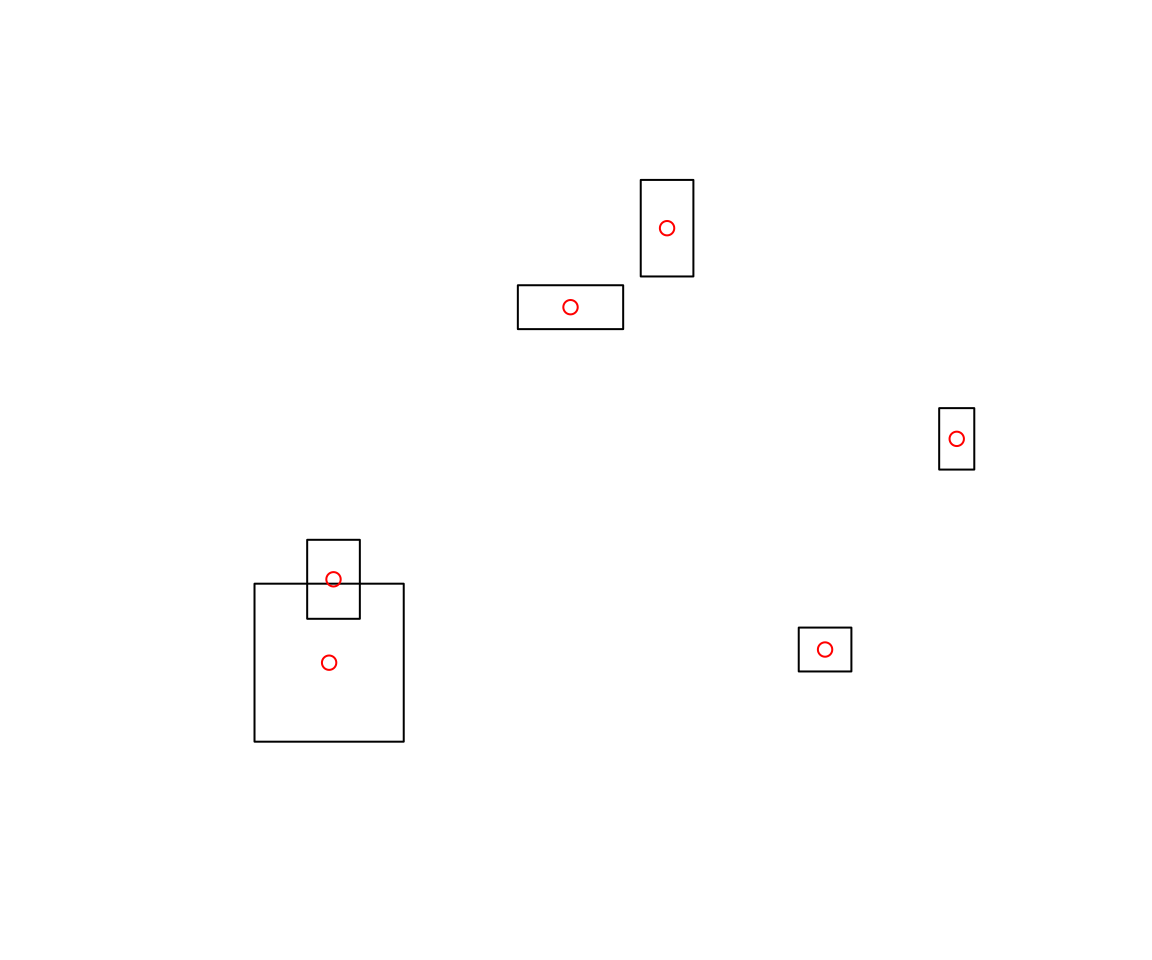
# Get random sample with density 0.02 pts per unit area
outRand <- getLandingsFromTarget(harvPoly, 0.02, sampleType = "random")
#> you have asked for > 0.001 pts per m2 which is > 1000 pts per km2 and may take a long time
prRand <- projectRoads(outRand, scen$cost.rast, scen$road.line)
#> 0s detected in weightRaster raster, these will be considered as existing roads

plot(scen$cost.rast, main = "Random Landings in Harvest Blocks",
     col = rastColours2)
plot(harvPoly, add = TRUE)
plot(prRand$roads, add = TRUE,  col = "grey50")
plot(outRand, col = "red", add = TRUE)
# Get regular sample with density 0.02 pts per unit area
outReg <- getLandingsFromTarget(harvPoly, 0.02, sampleType = "regular")
#> you have asked for > 0.001 pts per m2 which is > 1000 pts per km2 and may take a long time
prReg <- projectRoads(outReg, scen$cost.rast,scen$road.line)
#> 0s detected in weightRaster raster, these will be considered as existing roads


plot(scen$cost.rast, main = "Regular Landings in Harvest Blocks",
     col = rastColours2)
plot(harvPoly, add = TRUE)
plot(prReg$roads, add = TRUE, col = "grey50")
plot(outReg, col = "red", add = TRUE)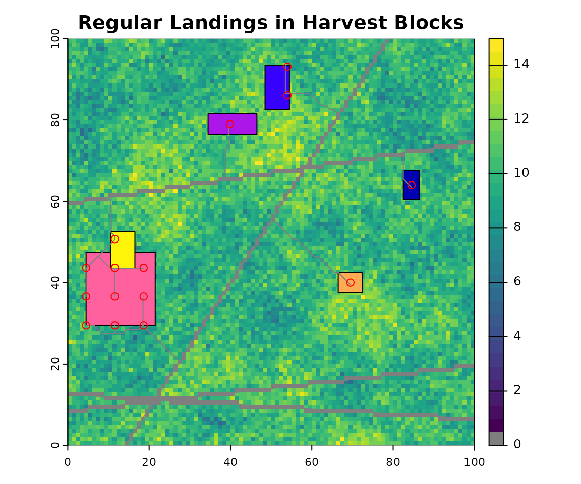
# clean up
par(oldpar)
Note
This vignette is partially copied from Kyle Lochhead & Tyler Muhly’s 2018 CLUS example