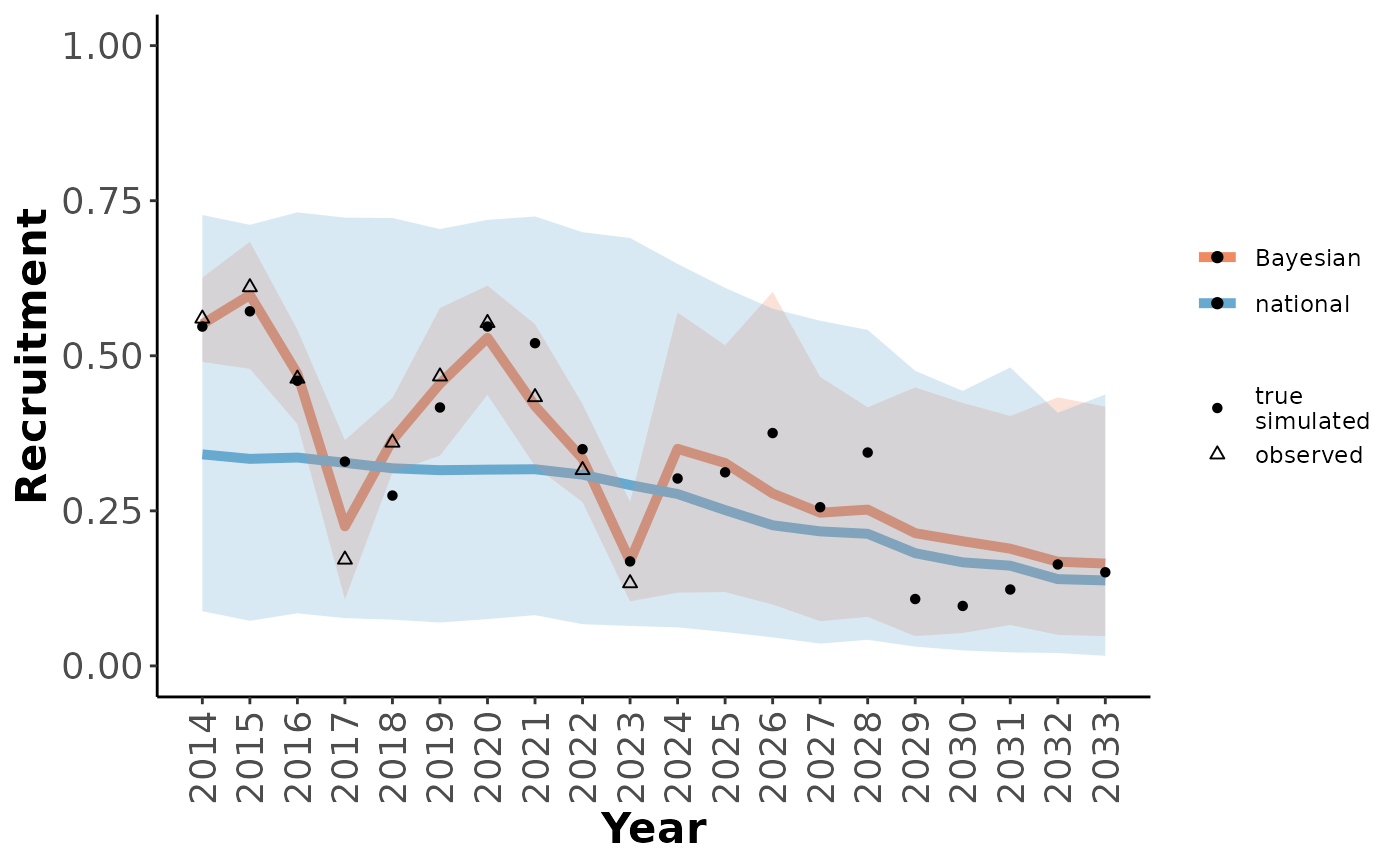
Plot Bayesian population model results

Plot Bayesian population model results, with (optionally) the distribution of outcomes from the initial model, local observations, and true local state for comparison.

Usage

plotRes(
  modTables,
  parameter,
  lowBound = 0,
  highBound = 1,
  facetVars = NULL,
  labFontSize = 14,
  legendPosition = "right",
  breakInterval = 1,
  typeLabels = c("Bayesian", "initial")
)

Arguments

modTables

list. A list of model results tables created using [getOutputTables()].

parameter

character. Which parameter to plot, if more than one, a list of plots is returned.

lowBound, highBound

numeric. Lower and upper y axis limits

facetVars

character. Optional. Vector of column names to facet by

labFontSize

numeric. Optional. Label font size if there are not facets. Font size is 10 pt if facets are used.

legendPosition

"bottom", "right", "left","top", or "none". Legend position.

breakInterval

number. How many years between x tick marks?

typeLabels

vector of two labels. Default c("Bayesian","initial"). Names of models to be compared.

Value

a ggplot object or list of ggplot objects if a vector of parameters was given.

See also

Caribou demography functions: bbouMakeSummaryTable(), caribouBayesianPM(), caribouPopGrowth(), caribouPopSimMCMC(), compositionBiasCorrection(), demographicCoefficients(), demographicProjectionApp(), demographicRates(), doSim(), getBBNationalInformativePriors(), getOutputTables(), getPriors(), getScenarioDefaults(), getSimsInitial(), getSimsNational(), popGrowthTableJohnsonECCC, runScnSet(), simulateObservations()

Examples

scns <- getScenarioDefaults(projYears = 10, obsYears = 10,
                            obsAnthroSlope = 1, projAnthroSlope = 5,
                            collarCount = 20, cowMult = 5)

simO <- simulateObservations(scns)

out <- caribouBayesianPM(surv_data = simO$simSurvObs, recruit_data = simO$simRecruitObs,
                          disturbance = simO$simDisturbance,
                          startYear = 2014, niters=10)
#> Compiling model graph
#>    Resolving undeclared variables
#>    Allocating nodes
#> Graph information:
#>    Observed stochastic nodes: 10
#>    Unobserved stochastic nodes: 33
#>    Total graph size: 665
#> 
#> Initializing model
#> 
#> Compiling model graph
#>    Resolving undeclared variables
#>    Allocating nodes
#> Graph information:
#>    Observed stochastic nodes: 29
#>    Unobserved stochastic nodes: 70
#>    Total graph size: 694
#> 
#> Initializing model
#> 

out_tbl <- getOutputTables(out, exData = simO$exData, paramTable = simO$paramTable,
                           simInitial = getSimsInitial())
#> Using saved object

plotRes(out_tbl, parameter = "Recruitment")